목차
앞서 대표적인 심층 생성 모델인 AutoRegressive Models (ARMs), Flow-based Models 두 가지를 살펴보았다. 하지만, (적어도 내가 연구하고 있는 분야에서는) 최근에는 VAE, Diffusion, GAN 기반의 모델이 활발하게 이용된다. 특히 diffusion의 우수한 성능은 따로 설명이 필요 없을 정도로 유명하고(실제로 세계적인 학회에 가면 과장 조금 보태서 30~40% 정도는 diffusion 관련 논문이 쏟아지고 있다.), VAE와 GAN을 기반으로 하는 다양한 우수한 성능을 보이는 모델이 나오고 있다.
VAE는 latent variable을 다룰 수 있다는 점에서 최근에는 생성모델 자체로 쓰이기 보다는 다양한 아키텍쳐들의 기반(base)으로 많이 사용되고 있다. 또한, diffusion은 다양한 관점에서 설명이 가능한데, VAE에서 활용되는 이론이 diffusion에서도 활용되며, 아예 diffusion을 hierarchical VAE로 보기도 한다. 따라서 책 'Deep Generative Modeling'을 참고하여 VAE에 대해 자세하게 공부하고, 정리해보려 한다.
이전 글에서는 VAE를 이해하는 데 필요한 기초 지식과 variational inference, ELBO 유도 과정을 자세히 살펴보았다.
Variational Auto-Encoder (VAE) 파헤치기! (1)
목차 앞서 대표적인 심층 생성 모델인 AutoRegressive Models (ARMs), Flow-based Models 두 가지를 살펴보았다. 하지만, (적어도 내가 연구하고 있는 분야에서는) 최근에는 VAE, Diffusion, GAN 기반의 모델이 활발
jjuke-brain.tistory.com
이번에는 VAE의 구성 요소를 간단히 정리하고, 학습 과정을 살펴보자. 그리고 간단한 구현 코드와 VAE 모델의 특징까지 알아보자.
Components of VAEs
Variational Auto-Encoders(VAE)는 Stochastic encoder \(q_\phi(\mathbf{z} \vert \mathbf{x})\)와 Stochastic decoder \(p(\mathbf{x} \vert \mathbf{z})\)로 구성된다. 또한, Marginal distribution (prior)는 \(p(\mathbf{z})\)로 주어진다.
VAE의 objective는 ELBO이며, 다음과 같이 표현된다. (유도 과정은 이전 글을 참조하자.)
\( \log p(\mathbf{x}) \geq \underbrace{ \mathbb{E}_{\mathbf{z} \sim q_\phi(\mathbf{z} \vert \mathbf{x})} \left[ \log p(\mathbf{x} \vert \mathbf{z}) \right] - \mathbb{E}_{\mathbf{z} \sim q_\phi(\mathbf{z} \vert \mathbf{x})} \left[ \log q_\phi(\mathbf{z} \vert \mathbf{x}) - \log p(\mathbf{z}) \right]}_{\text{ELBO}} \)
Parameterization of Distributions
Encoder와 decoder는 Neural network를 활용하여 parameterize한다.
VAE를 모델링 할 때, distribution 선택이 자유롭지만 domain에 따른 차원 등을 잘 고려해야 한다.
예를 들어, image의 경우 \(\mathbf{x} \in \{0, 1, \dots, 255 \}^D\)로 주어지므로, Normal distribution은 활용할 수 없다. 따라서 아래와 같이 categorical distribution을 사용해야 한다.
\( p_\theta(\mathbf{x} \vert \mathbf{z}) = \operatorname{Categorical}(\mathbf{x} \vert \theta(\mathbf{z})) \)
여기서, \(\theta(\mathbf{z}) = \operatorname{softmax}(\operatorname{NN}(\mathbf{z}))\)이며, \(\operatorname{NN}\)은 MLP, CNN, RNN 등의 neural network를 의미한다.
Variational posterior와 prior의 distribution은 보통 가장 간단한 형태인 Gaussian을 사용한다.
\( q_\phi(\mathbf{z} \vert \mathbf{x}) = \mathcal{N}\left( \mathbf{z} \vert \boldsymbol{\mu}_\phi(\mathbf{x}), \boldsymbol{\Sigma}_\phi(\mathbf{x}) \right) \)
\( p(\mathbf{z}) = \mathcal{N}(\mathbf{z} \vert \boldsymbol{0}, \mathbf{I}) \)
이때 \(\mathbf{z} \in \mathbb{R}^M\)는 continuous random variable로 이루어진 벡터이며, \(\boldsymbol{\mu}_\phi(\mathbf{x}), \boldsymbol{\Sigma}_\phi(\mathbf{x})\)는 neural network의 output이다. 실제 구현할 때에는 2\(M\)개의 값을 반환한다. (mean, variance 각각 \(M\)개)
아래부터는 mean, variance의 표기를 간단하게 \(\mu\), \(\sigma\)로 하겠다.
Reparameterization Trick
ELBO를 통해 log-likelihood를 근사했지만, 여전히 기댓값 계산, 즉 integral 계산은 어렵다.
따라서 계산 불가능한 식을 근사하기 위한 Monte Carlo approximation(MC-approximation, 자세한 내용은 이전 글 참조)을 사용하되, prior \(p(\mathbf{z})\) 대신 variational posterior \(q_\phi(\mathbf{z} \vert \mathbf{x})\)에서 샘플링한다.
이 방법의 장점은 variational posterior가 prior보다 더 많은 probability mass를 더 작은 region에 할당하기 때문에, variance 측면에서 거의 deterministic하게 근사할 수 있다는 것이다. 그러나, approximation의 variance 문제는 여전히 존재한다. (샘플링한 \(\mathbf{z} \sim q_\phi(\mathbf{z} \vert \mathbf{x})\)를 ELBO에 대입하고 neural network \(\phi\)에 대한 gradient의 variance를 계산해보면 매우 큰 값이 나온다.)
이 문제를 해결하기 위해 reparameterization trick을 사용한다.
Reparameterization이란, 어떤 random variable을 간단한 distribution에서 얻은 독립변수들의 primitive transformation으로 표현하는 방법이다.
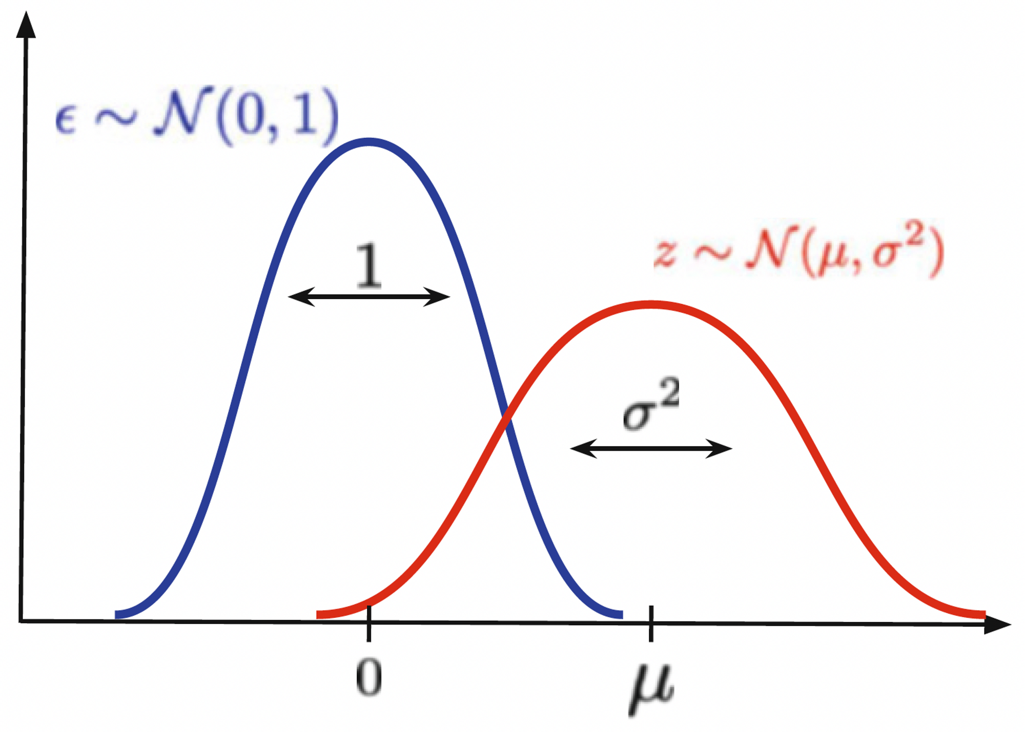
예를 들어, Gaussian random variable \(z \sim \mathcal{N}(\mu, \sigma^2)\)와 independent random variable \(\epsilon \sim \mathcal{N}(\epsilon \vert 0, 1)\)에 대해 다음이 성립한다.
\( z = \mu + \sigma \cdot \epsilon \)
즉, standard Gaussian에서 \(\epsilon\)을 샘플링하여 transformation을 적용하면 \(\mathcal{N}(z \vert \mu, \sigma^2)\)에서 얻은 샘플을 얻는 것과 같다.
이는 Fig 1에서 볼 수 있듯이 \(\epsilon \sim \mathcal{N}(\epsilon \vert 0, 1)\)을 \(sigma\)만큼 scaling하고 \(\mu\)만큼 shifting하여 원하는 샘플을 얻는 개념으로 볼 수 있다.
그렇다면 VAE에서는 reparameterization trick을 어떻게 사용할까?
Encoder \(q_\phi(\mathbf{z} \vert \mathbf{x})\)에서 Gaussian distribution의 reparameterization을 활용하여 gradient의 variance를 크게 줄일 수 있다. Randomness가 독립적인 값인 \(\epsilon\)에서 오고, neural network라는 deterministic function에 대해 gradient를 계산하기 때문이다.
게다가, VAE는 stochastic gradient descent 방식으로 학습되기 때문에, 학습 중에 한 번만 \(\mathbf{z}\)를 샘플링해도 된다!
VAE Implementation (Example)
이제 예시와 함께 VAE의 학습이 실제로 어떻게 이루어지는지 알아보자.
Encoder, Prior, and Decoder
VAE에서 활용할 distributions는 다음과 같다고 가정하자.
- Encoder \( q_\phi(\mathbf{z} \vert \mathbf{x}) = \mathcal{N} \left( \mathbf{z} \vert \mu_\phi(\mathbf{x}), \sigma_\phi^2(\mathbf{x}) \right) \)
- Prior \( p(\mathbf{z}) = \mathcal{N}(\mathbf{z} \vert \boldsymbol{0}, \mathbf{I}) \)
- Decoder \( p_\theta(\mathbf{x} \vert \mathbf{z}) = \operatorname{Categorical}(\mathbf{x} \vert \theta(\mathbf{z})) \)
그리고 input data \(\mathbf{x} \in \mathcal{X}^{D \times L}\)는 categorical distribution을 따른다고 가정하자. \(D\)는 pixel 개수 (예를 들어 224 by 224 image이면 \(D=50176\)), \(L\)은 pixel의 가능한 값 개수(예를 들어 8bit이면 0 ~ 255, 즉 256)이다.
VAE에서 활용될 수 있는 encoder, decoder network를 알아보자.
Encoder network는 다음과 같이 정의된다.
\( \begin{align*} \mathbf{x} \in \mathbf{X}^D \rightarrow &\operatorname{Linear}(D, 256) \rightarrow \operatorname{LeakyReLU} \rightarrow \\ &\operatorname{Linear}(256, 2 \cdot M) \rightarrow \operatorname{split} \rightarrow \mu \in \mathbb{R}^M, \; \log \sigma^2 \in \mathbb{R}^M \end{align*} \)
여기서, 2M개 중 M개의 값은 mean을 나타내고, 나머지 M개는 log variance 추정에 활용된다. variance는 양수여야 하는데 network가 추정하는 값은 실수이므로, log variance를 추정한다.
Decoder network는 다음과 같이 정의된다.
\( \begin{align*} \mathbf{z} \in \mathbb{R}^M \rightarrow & \operatorname{Linear}(M, 256) \rightarrow \operatorname{LeakyReLU} \rightarrow \\ & \operatorname{Linear}(256, D \cdot L) \rightarrow \operatorname{reshape} \rightarrow \operatorname{softmax} \rightarrow \theta \in [0, 1]^{D \times L} \end{align*} \)
Input은 categorical distribution을 따르기 때문에, decoder network는 확률 \(D \cdot L\)개를 출력한다. Output tensor의 형태는 \(B, D, L\)로 reshape되어야 하며, 여기서 \(B\)는 batch size를 나타낸다. Softmax 함수를 통해 확률 값을 얻는다.
이를 PyTorch 코드로 작성하면 다음과 같다.
class Encoder(nn.Module):
    def __init__(self, encoder_net):
        super(Encoder, self).__init__()
        self.encoder = encoder_net

    @staticmethod
    def reparameterization(mu, log_var):
        std = torch.exp(0.5*log_var)
        eps = torch.randn_like(std)
        return mu + std * eps

    def encode(self, x):
        h_e = self.encoder(x) # 2M size output
        mu_e, log_var_e = torch.chunk(h_e, 2, dim=1)
        return mu_e, log_var_e

    def sample(self, x=None, mu_e=None, log_var_e=None):
        if (mu_e is None) and (log_var_e is None):
            mu_e, log_var_e = self.encode(x)
        else:
            if (mu_e is None) or (log_var_e is None):
                raise ValueError('mu and log variance should not be None.')
				z = self.reparameterization(mu_e, log_var_e)
				return z

		def log_prob(self, x=None, mu_e=None, log_var_e=None, z=None):
				if x is not None:
						# calculate corresponding sample
						mu_e, log_var_e = self.encode(x)
						z = self.sample(mu_e=mu_e, log_var_e=log_var_e)
				else:
						if (mu_e is None) or (log_var_e is None) or (z is None):
								raise ValueError('mu, log variance, z should not be None.')

				return log_normal_diag(z, mu_e, log_var_e)

		def forward(self, x, type='log_prob'):
				assert type in ['encode', 'log_prob'], 'Type could be either encode or log_prob'

				if type == 'log_prob':
						return self.log_prob(x)
				else: # type == 'encode'
						return self.sample(x)
# Prior : simple standard Gaussian
class Prior(nn.Module):
		def __init__(self, L):
				super(Prior, self).__init__()
				self.L = L

		def sample(self, batch_size):
				z = torchrandn((batch_size, self.L))
				return z

		def log_prob(self, z):
				return log_standard_normal(z)
class Decoder(nn.Module):
		def __init__(self, decoder_net,
								 distribution='categorical', num_vals=None):
				super(Decoder, self).__init__()

				self.decoder = decoder_net
				self.distribution = distribution
				self.num_vals = num_vals

		def decode(self, z):
				h_d = self.decoder(z)
				if self.distribution == 'categorical':
						b = h_d.shape[0] # batch size
						d = h_d.shape[1] // self.num_vals # D
						h_d = h_d.view(b, d, self.num_vals) # (B,D,L)
						mu_d = torch.softmax(h_d, 2) # (B,D,L)
						return [mu_d]
				else:
						pass # we can use other distributions!

		def sample(self, z):
				outs = self.decode(z)
				if self.distribution == 'categorical':
						mu_d = outs[0] # (B,D,L)
						b, m = mu_d.shape[0], mu_d.shape[1]

						mu_d = mu_d.view(mu_d.shape[0], -1, self.num_vals) # (B,D,L)
						p = mu_d.view(-1, self.num_vals) # (B*D,L)
						x_new = torch.multinomial(p, num_samples=1).view(b,m) # (B*D,1) → (B, D)
				else:
						pass # we can use other distributions!

				return x_new

		def log_prob(self, x, z):
				outs = self.decode(z)
				if self.distribution == 'categorical':
						mu_d = outs[0]
						log_p = log_categorical(x, mu_d, num_classes=self.num_vals,
																		reduction='sum', dim=-1).sum(-1)
				else:
						pass # we can use other distributions!

				return log_p

		def forward(self, z, x=None, type='log_prob'):
				assert type in ['decoder', 'log_prob'], 'Type should be either decode or log_prob'

				if type == 'log_prob':
						return self.log_prob(x, z)
				else:
						return self.sample(x)
\(\mathbf{x}\) → encoder → bottleneck (\(\mathbf{z}\)) → decoder → \(\mathbf{x}\) 형태가 가능한 어떤 neural network던 encoder, decoder에 활용이 가능하다.
Training
다음으로, training objective를 살펴보자.
Variational posterior로부터 reparameterize하여 얻은 샘플은 다음과 같다.
\( \mathbf{z}_{\phi, n} = \mu_\phi(\mathbf{x}_n) + \sigma_\phi(\mathbf{x}_n) \odot \epsilon \)
학습 과정에서 최소화할 loss는 negative ELBO이며, 이는 다음과 같이 표현한다.
\( \begin{align*} -\operatorname{ELBO}(\mathcal{D}; \theta, \phi) = - \sum\limits_{n=1}^N & \log \operatorname{Categorical}(\mathbf{x}_n \vert \theta(\mathbf{z}_{\phi,n})) + \\ & \left[ - \log \mathcal{N}\left( \mathbf{z}_{\phi,n} \vert \mu_\phi(\mathbf{x}_n), \sigma_\phi^2(\mathbf{x}_n) \right) + \log \mathcal{N}(\mathbf{z}_{\phi,n} \vert \operatorname{0}, \mathbf{I}) \right] \end{align*} \)
이전에 유도한 ELBO와 비교해보면, 결국 위 식은 encoder, decoder, prior를 distribution으로 표현한, 같은 표현이라는 것을 알 수 있다.
\( \log p(\mathbf{x}) = \underbrace{\mathbb{E}_{\mathbf{z} \sim q_\phi(\mathbf{z} \vert \mathbf{x})} \left[ \log p(\mathbf{x} \vert \mathbf{z}) \right] - D_\text{KL} \left[ q_\phi(\mathbf{z} \vert \mathbf{x}) \Vert p(\mathbf{z}) \right]}_{\text{ELBO}} + \underbrace{D_\text{KL} \left[ q_\phi(\mathbf{z} \vert \mathbf{x}) \Vert p(\mathbf{z} \vert \mathbf{x}) \right]}_{\geq 0} \)
Training 과정은 다음과 같다.
- 입력 \(\mathbf{x}_n\)을 encoder network에 입력하여 mean \(\mu_\phi(\mathbf{x}_n)\)과 log variance \(\log \sigma_\phi^2(\mathbf{x}_n)\)을 얻는다.
- Reparameterization trick을 사용하여 standard Gaussian에서 얻은 \(\epsilon\)을 사용하여 \(\mathbf{z}_{\phi,n}\)을 계산한다.
- 샘플 \(\mathbf{z}_{\phi,n}\)을 decoder network에 입력하여 probabilities \(\theta(\mathbf{z}_{\phi,n})\)을 얻는다.
- \(\mathbf{x}_n, \mathbf{z}_{\phi,n}\), \(\mu_\phi(\mathbf{x}_n)\), \(\log \sigma_\phi^2(\mathbf{x}_n)\)을 사용하여 ELBO, 즉 loss를 계산한다.
따라서 VAE 코드는 다음과 같이 작성해볼 수 있다.
class VAE(nn.Module):
		def __init__(self, encoder_net, decoder_net, num_vals=256,
								 L=16, likelihood_type='categorical'):
				super(VAE, self).__init__()

				self.encoder = Encoder(encoder_net=encoder_net)
				self.decoder = Decoder(decoder_net=decoder_net,
															 distribution=likelihood_type, num_vals=num_vals)
				self.prior = Prior(L=L)

				self.num_vals = num_vals
				self.likelihood_type = likelihood_type

		def forward(self, x, reduction='avg'):
				# encoder
				mu_e, log_var_e = self.encoder.encode(x)
				z = self.encoder.sample(mu_e=mu_e, log_var_e=log_var_e)

				# ELBO
				recon = self.decoder.log_prob(x, z)
				kl = (self.prior.log_prob(z) - self.encoder.log_prob(mu_e=mu_e,
							log_var_e=log_var_e, z=z)).sum(-1)

				if reduction == 'sum':
						return -(recon + kl).sum()
				else:
						return -(recon + kl).mean()

		def sample(self, batch_size=64):
				z = self.prior.sample(batch_size=batch_size)
				return self.decoder.sample(z)
Strengths and Weaknesses of the VAEs
이제까지 deep generative model 중 AutoRegressive Models(ARMs), Flow-based Models, Variational AutoEncoders(VAEs)를 알아보았다.
VAE와 flow-based model을 비교하면, VAE는 Neural network에 invertible한 함수를 사용하지 않아도 되므로 encoder와 decoder에 어떤 아키텍쳐든 활용할 수 있다는 장점을 갖는다.
VAE와 ARM을 비교하면, VAE는 저차원의 data representation(latent variable)을 학습하고, control할 수 있다.
그러나, VAEs는 몇 가지 문제점을 갖고 있다.
- 실제 log-likelihood와 ELBO 사이에는 차이가 있다(ELBO의 유도 과정에서 생략했던 KL divergence term). ARM, Flow-based Model에 비해서는 학습 및 평가 과정이 복잡하고, 불안정하다.
- Posterior collapse
- Decoder가 너무 강력해져서 latent variable \(\mathbf{z}\)를 noise로 간주해버린다. ELBO의 regularization term \( D_\text{KL} \left[ q_\phi(\mathbf{z} \vert \mathbf{x}) \Vert p(\mathbf{z}) \right] \)에 의해 encoder의 output distribution이 standard Gaussian prior에 너무 가까워진 현상이다.
- 이에 따라 latent variable 자체가 의미가 없어지고, reconstruction 성능이 나빠지며, 생성 결과의 diversity가 떨어진다.
- Hole problem : Aggregated posterior \( q_\phi(\mathbf{z}) = \cfrac{1}{N} \sum\limits_{n} q_\phi(\mathbf{z} \vert \mathbf{x}_n) \)과 prior \(p(\mathbf{z})\)가 서로 맞지 않아(mismatch) hole이 생기는 경우이다.
- Prior에서는 높은 확률이 aggregated posterior에서는 낮을 수 있다. (반대의 경우도 가능)
- Hole에서 샘플링한 latent variable이 비현실적이게 되고, 이것으로 decoding한 결과가 매우 낮은 quality를 가진다.
- Out-of-distribution problem : 서로 다른 distribution을 갖는 sample은 전혀 생성하지 못하는 문제이다.
- 모든 심층 생성 모델들이 공통적으로 갖고 있는 문제점이다.


최근댓글