Xiang Gao, Tao Zhang 저자의 'Introduction to Visual SLAM from Theory to Practice' 책을 통해 SLAM에 대해 공부한 내용을 기록하고자 한다.
책의 내용은 주로 'SLAM의 기초 이론', 'system architecture', 'mainstream module'을 다룬다.
Lie Group, Lie Algebra의 기본 개념을 알고싶다면 이전 포스팅을 참조하자.
https://jjuke-brain.tistory.com/entry/Lie-Group-and-Lie-Algebra
Lie Group and Lie Algebra (1) - 정의, so(3), se(3), Exponential Mapping, Logarithmic Mapping
Xiang Gao, Tao Zhang 저자의 'Introduction to Visual SLAM from Theory to Practice' 책을 통해 SLAM에 대해 공부한 내용을 기록하고자 한다. 책의 내용은 주로 'SLAM의 기초 이론', 'system architecture', 'ma..
jjuke-brain.tistory.com
포스팅에는 기초 이론만 다룰 것이며, 실습을 해보고 싶다면 다음 github를 참조하자.
https://github.com/gaoxiang12/slambook2
GitHub - gaoxiang12/slambook2: edition 2 of the slambook
edition 2 of the slambook. Contribute to gaoxiang12/slambook2 development by creating an account on GitHub.
github.com
목차
Lie algebra를 배우는 주요 이유는 바로 optimization(최적화)를 위해서이다. 이 과정에서는 도함수가 필수적으로 필요하다.
이와 관련된 개념을 알아보자.
Lie Algebra Derivation and Perturbation Model
BCH Formula and its Approximation
앞선 포스팅에서 Lie group과 Lie algebra간의 관계를 이해해 보았었는데, 그를 바탕으로 과연 다음 수식들이 맞을지 판단해보자.
\( \text{exp}(\boldsymbol{\phi}_1^\wedge) \text{exp}(\boldsymbol{\phi}_2^\wedge) = \text{exp} \left( \left( \boldsymbol{\phi}_1 + \boldsymbol{\phi_2} \right)^\wedge \right) ? \)
\( \ln{\left( \text{exp}(\mathbf{A}) \text{exp} (\mathbf{B}) \right)} = \mathbf{A + B} ? \)
만약 \( \boldsymbol{\phi_1, \phi_2}, \mathbf{A, B} \)가 스칼라였다면 당연히 맞겠지만, 우리는 지금 matrix를 다루고 있으므로 애매하다.
사실 위 두 식은 matrix의 경우 틀린 식이다.
Product 연산에 대한 complete form은 Baker-Campbell-Hausdorff formula (BCH formula)로 주어진다.
Complete form은 너무 복잡하므로 거기서 확장된 처음 몇 term들만 살펴보자.
\( \ln{\left( \text{exp}(\mathbf{A}) \text{exp} (\mathbf{B}) \right)} = \mathbf{A} + \mathbf{B} + \frac{1}{2} \mathbf{[A, B]} + \frac{1}{12} \mathbf{[A, [A, B]]} - \frac{1}{12} \mathbf{[B, [A, B]]} + \dots \)
이때 '[]'는 Lie bracket을 나타낸다.
BCH formula는 이렇게 두 matrix간의 product 연산을 나타낸다. (scalar form에 비해 Lie bracket이 더 많다.)
이번에는 좀 더 특별한 경우인 \(\boldsymbol{\phi_1, \phi_2}\)가 작을 때 \(\text{SO}(3)\)와 \( \ln{(\text{exp}(\boldsymbol{\phi}_1^\wedge)\text{exp}(\boldsymbol{\phi}_2^\wedge))^\vee} \)를 고려해보자.
도함수를 구할 때 2차식 이상의 작은 값은 무시된다. 이때 BCH를 다음과 같이 (선형)근사화할 수 있다.
\( \ln{(\text{exp}(\boldsymbol{\phi}_1^\wedge)\text{exp}(\boldsymbol{\phi}_2^\wedge))^\vee} \approx \begin{cases} \mathbf{J}_l (\boldsymbol{\phi}_2)^{-1} \boldsymbol{\phi}_1 + \boldsymbol{\phi}_2 \text{when }\boldsymbol{\phi}_1 \text{is a small amount} \\ \mathbf{J}_r (\boldsymbol{\phi}_1)^{-1} \boldsymbol{\phi}_2 + \boldsymbol{\phi}_1 \text{when }\boldsymbol{\phi}_2 \text{is a small amount} \end{cases} \)
[Ref] Right and Left Matrix Multiplication
근사 과정을 자세히 살펴보기 전에, right multiplication과 left multiplication을 간단히 살펴보자.
Right-multiplication과 left-multiplication은 단순히 행렬곱(Matrix multiplication)을 특정 형태로 나타내는 것이다.
- Right-multiplication : Combination of columns
- Left-multiplication : Combination of rows
예를 들어, 어떤 행렬과 column vector의 곱이 다음과 같이 존재한다.
\( \begin{bmatrix} x_1 & y_1 & z_1 \\ x_2 & y_2 & z_2 \\ x_3 & y_3 & z_3 \end{bmatrix} \begin{pmatrix} a \\ b \\ c \end{pmatrix} = \begin{pmatrix} a x_1 + b y_1 + c z_1 \\ a x_2 + b y_2 + c z_2 \\ a x_2 + b y_2 + c z_2 \end{pmatrix} \)
어떤 행렬과 열벡터의 right-multiplying은 해당 행렬의 열의 선형 결합과 같다.
linear algebra에서 배운 linear equation 형태와 같다.
이때, matrix의 column을 기준으로 곱해지는 과정을 생각해보면, 다음과 같이 그림으로 나타낼 수 있다.
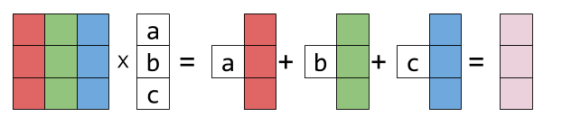
첫 번째 column \( \begin{bmatrix} x_1 \\ x_2 \\ x_3 \end{bmatrix} \)은 빨간 색, 두 번째 column \( \begin{bmatrix} y_1 \\ y_2 \\ y_3 \end{bmatrix} \)은 초록색, 세 번째 column \( \begin{bmatrix} z_1 \\ z_2 \\ z_3 \end{bmatrix} \)은 파란 색으로 나타냈다.
곱셈 과정을 흰 배경의 박스, 즉 스칼라(coefficients)와 각 column vector의 곱의 선형 결합으로 나타낸 것이다.
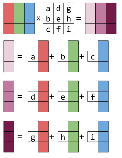
행렬과 행렬의 right-multiplication도 그림을 통해 쉽게 확장하여 생각해볼 수 있다.
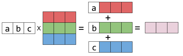
Left-multiplication은 반대로 어떤 행렬을 행벡터로 곱하는 것을 말한다. (곱하는 벡터의 위치가 왼쪽)
다음 예시를 보자.
\( \begin{pmatrix} a & b & c \end{pmatrix} \begin{bmatrix} x_1 & y_1 & z_1 \\ x_2 & y_2 & z_2 \\ x_3 & y_3 & z_3 \end{bmatrix} = \begin{pmatrix} a x_1 + b x_2 + c x_3 & a y_1 + b y_2 + c y_3 & a z_1 + a z_2 + a z_3 \end{pmatrix} \)
어떤 행렬과 행벡터의 left-multiplying은 해당 행렬의 행의 선형 결합과 같다.
그림으로는 다음과 같이 나타낼 수 있다.
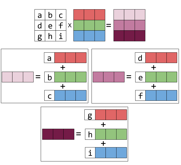
행렬과 행렬의 left-multiplication 또한 그림으로 나타내면 다음과 같다.
이제 BCH의 근사화로 다시 돌아와보자.
\( \ln{(\text{exp}(\boldsymbol{\phi}_1^\wedge)\text{exp}(\boldsymbol{\phi}_2^\wedge))^\vee} \approx \begin{cases} \mathbf{J}_l (\boldsymbol{\phi}_2)^{-1} \boldsymbol{\phi}_1 + \boldsymbol{\phi}_2 \quad \text{when }\boldsymbol{\phi}_1 \text{is a small amount} \\ \mathbf{J}_r (\boldsymbol{\phi}_1)^{-1} \boldsymbol{\phi}_2 + \boldsymbol{\phi}_1 \quad \text{when }\boldsymbol{\phi}_2 \text{is a small amount} \end{cases} \)
먼저 첫 번째(위) 식의 의미를 살펴보자.
매우 작은 회전에 대한 rotation matrix인 \( \mathbf{R}_1 \)을 \( \mathbf{R}_2 \)로 left-multiplying한 결과(\( \mathbf{R}_1, \mathbf{R}_2 \)의 Lie algebra는 각각 \( \boldsymbol{\phi}_1, \boldsymbol{\phi}_2 \))는 \( \mathfrak{so}(3) \)에서 \( \mathbf{J}_l (\boldsymbol{\phi}_2)^{-1} \boldsymbol{\phi}_1 \) term을 \( \boldsymbol{\phi}_2 \)에 더하는 것으로 근사화될 수 있다는 것이다.
두 번째(아래) 식도 마찬가지 개념이다.
\( \mathbf{R}_1 \)이 \( \mathbf{R}_2 \)라는 작은 rotation을 표현하는 matrix에 의해 right-multiplication되었을 때의 approximation을 나타낸다.
따라서, BCH approximation을 적용하게 되면 Lie algebra는 left-multiplying approximation과 right-multiplying approximation으로 나누어진다.
실제 left model과 right model 중 어떤 것을 사용할 지를 골라야 한다.
이 책에서는 left multiplication을 예시로 취하고 있다.
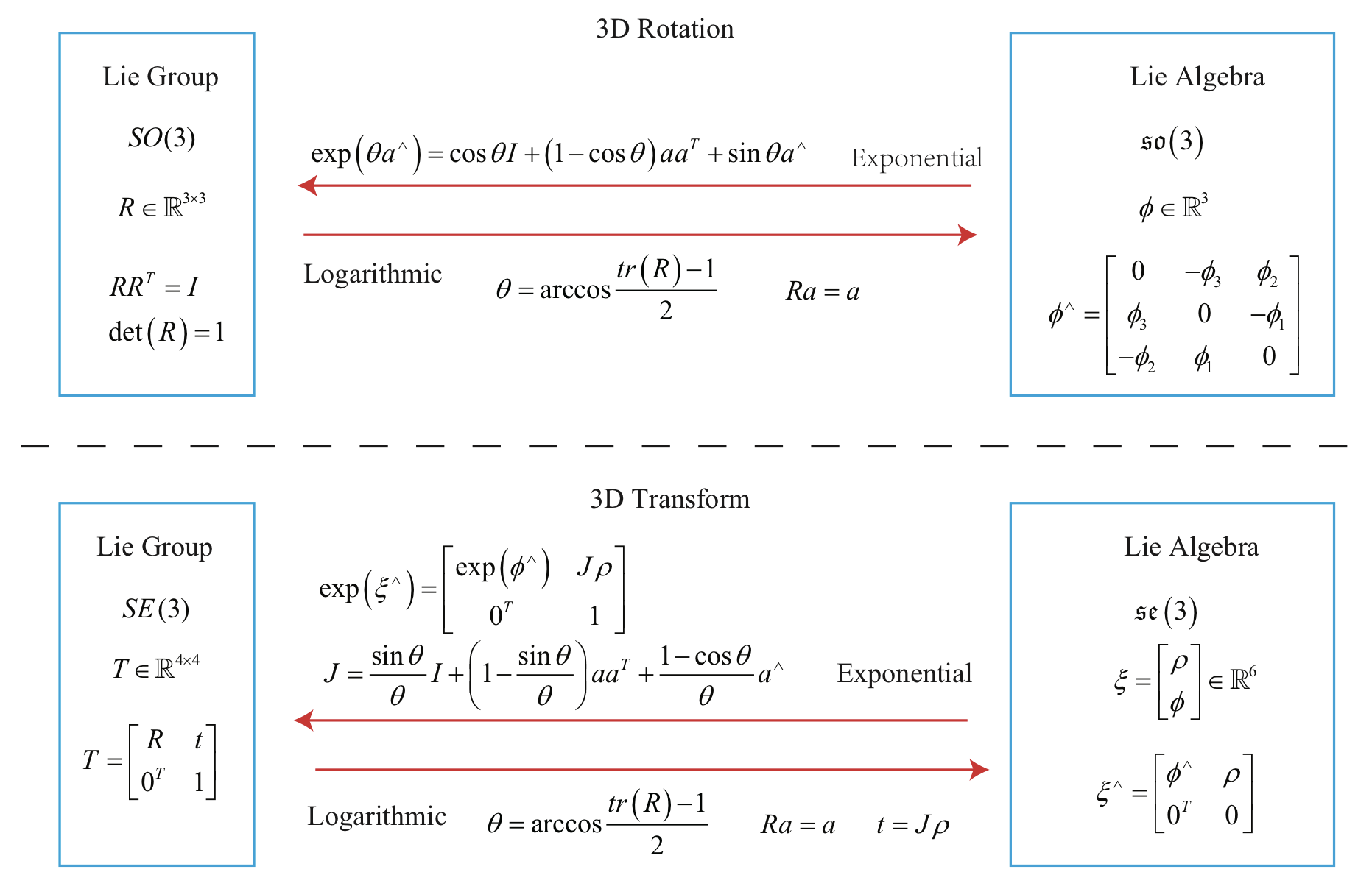
Left model에서의 jacobian \( \mathbf{J}_l \)은 위와 같은 Lie group과 Lie algebra 간의 관계에 의해 다음의 형태를 가질 것이다. (자세한 내용은 이전 포스팅을 참조하자.)
\( \mathbf{J}_l = \mathbf{J} = \frac{\sin\theta}{\theta} \mathbf{I} + \left( 1 - \frac{\sin\theta}{\theta} \right) \mathbf{aa}^T + \frac{1 - \cos\theta}{\theta} \mathbf{a}^\wedge \)
그리고 inverse(역)는 다음과 같다.
\( \mathbf{J}_l^{-1} = \frac{\theta}{2} \cot{\frac{\theta}{2}} \mathbf{I} + \left( 1 - \frac{\theta}{2} \cot{\frac{\theta}{2}} \right) \mathbf{aa}^T - \frac{\theta}{2} \mathbf{a}^\wedge \)
\( \theta \)가 0이면 \( \mathbf{J}_l, \mathbf{J}_l^{-1} \) 모두 identity matrix일 것이고, 0이 아니면 right jacobian \( \mathbf{J}_r \)을 얻기 위해 인자에 -부호만 붙여주면 된다.
\( \mathbf{J}_r(\boldsymbol{\phi}) = \mathbf{J}_l (- \boldsymbol{\phi}) \)
이러한 방법으로, Lie group multiplication과 Lie algebra addition간의 관계를 알게 되었다.
BCH approximation을 정리해보자.
rotation \( \mathbf{R} \)이 있다고 가정했을 때, 이에 대응되는 Lie algebra는 \( \boldsymbol{\phi} \)이다. 왼쪽으로 아주 작은 회전(작은 변화 - perturbation) \( \Delta \mathbf{R} \)을 주면, 이에 따라 Lie algebra 또한 \( \Delta \boldsymbol{\phi} \)만큼 변하게 된다. 그러면 Lie group에서는 그 결과가 \( \Delta \mathbf{R \cdot R} \)로 나타나는데, Lie algebra에서는 BCH approximation에 따라 \( \mathbf{J}_l^{-1} (\boldsymbol{\phi}) \Delta \boldsymbol{\phi} + \boldsymbol{\phi} \)로 나타난다.
이를 수식으로 나타내면 다음과 같다.
\( \text{exp}(\Delta \boldsymbol{\phi}^\wedge) \text{exp}(\boldsymbol{\phi}^\wedge) = \text{exp} \left( \left( \boldsymbol{\phi} + \mathbf{J}_l^{-1} (\boldsymbol{\phi}) \Delta \boldsymbol{\phi} \right)^\wedge \right) \)
역으로, Lie algebra의 addition으로 Lie group의 multiplication을 근사화하기 위해서는 다음 수식을 사용한다.
\( \text{exp} \left( \left( \boldsymbol{\phi} + \Delta \boldsymbol{\phi} \right)^\wedge \right) = \text{exp} \left( \left( \mathbf{J}_l \Delta \boldsymbol{\phi} \right)^\wedge \right) \text{exp}(\boldsymbol{\phi}^\wedge) = \text{exp} (\boldsymbol{\phi}^\wedge) \text{exp} \left( \left( \mathbf{J}_r \Delta \boldsymbol{\phi} \right)^\wedge \right) \)
Lie algebra의 미적분에도 이 개념이 기초로 사용된다.
\( \text{SE}(3) \)에도 비슷한 BCH approximation이 사용된다.
\( \text{exp}(\Delta \boldsymbol{\xi}^\wedge) \text{exp}(\boldsymbol{\xi}^\wedge) \approx \text{exp} \left( \left( \mathcal{J}_l^{-1} \Delta \boldsymbol{\xi} + \boldsymbol{\xi} \right)^\wedge \right) \)
\( \text{exp}(\boldsymbol{\xi}^\wedge) \text{exp}(\Delta \boldsymbol{\xi}^\wedge) \approx \text{exp} \left( \left( \mathcal{J}_r^{-1} \Delta \boldsymbol{\xi} + \boldsymbol{\xi} \right)^\wedge \right) \)
\( \mathcal{J}_l, \mathcal{J}_r \)은 좀 더 복잡한 6 × 6 matrix이다. 이 책에서 두 jacobian matrix를 계산에 사용할 일은 없기 때문에 자세한 내용은 생략한다.
Derivative on \( \text{SO}(3) \)
이제 optimization의 주요 과정인 미분을 계산하는 방법을 알아보자.
목적 함수(target function)는 rotation 또는 transform과 관련되어있는데, SLAM 문제를 해결할 때 최적화를 위한 이러한 함수를 활용하게 된다.
어떤 로봇의 \( \text{SO}(3) \) 또는 \( \text{SE}(3) \)로 표현된 pose를 추정한다고 가정해보자.
로봇은 world coordinate내의 \( \mathbf{p} \) 점을 관측하고, 관측 데이터(observation data) \( \mathbf{z} \)를 발생시킬 것이다.
이 과정을 수식으로 표현하면 다음과 같다.
\( \mathbf{z = Tp + w} \)
여기서 \( \mathbf{w} \)는 noise이다.(unknown)
noise때문에 실제 관측 데이터는 관측한 model으로부터 계산한 값과 미세하게 차이를 보일 것이다.
따라서 실제 값과 계산한 값(predicted observation) 사이의 차이인 에러 \( \mathbf{e} \)를 다음과 같이 나타낼 수 있다.
\( \mathbf{e = z - Tp} \)
총 \(N\)개의 점을 관측한다고 한다면, error를 최소화하는 최적의 \( \mathbf{T} \)를 다음 식을 통해 찾을 수 있다.
\( \underset{\mathbf{T}}{\min} J(\mathbf{T}) = \sum\limits_{i=1}^{N} \lVert \mathbf{z}_i - \mathbf{T} \mathbf{p}_i \rVert_2^2 \)
위와 같은 least square problem(optimized problem)을 풀기 위해서는 \( \mathbf{T} \)에 대한 \(J\)의 도함수(derivative)를 구할 필요가 있다.
최적화 문제를 푸는 과정은 이후에 다루도록 하고, 여기서는 rotation 또는 transform을 변수로 갖는 함수를 명확하게 알아보자.
하지만 이전에 언급했듯이, \( \text{SO}(3) \)와 \( \text{SE}(3) \)는 (group이므로) addition 연산이 존재하지 않기 때문에 일반적인 형태로는 derivative를 정의해줄 수 없다.
\( \mathbf{R, T} \)를 일반적인 matrix로 취급한다면, optimization 과정에서 제한이 많을 것이다. 하지만, Lie algebra의 관점에서는 벡터로 이루어져있기 때문에 addition operation이 존재한다.
따라서, Lie algebra를 사용하여 다음과 같은 두 가지 방법으로 derivation 문제를 해결할 수 있다.
- Lie algebra에 아주 작은(infinitesimal) 값을 더한다고 가정하고, object function의 변화량을 계산한다.
- Lie group에 left multiplication 혹은 right multiplication을 통해 Lie algebra로 표현된 아주 작은 양의 perturbation을 곱하여 이러한 perturbation에 대한 derivative를 계산한다. (Left Perturbation Model / Right Perturbation Model)
첫 번째 방법은 Lie algebra의 일반적인 derivation model이고, 두 번째 방법은 perturbation model에 해당한다.
Derivation Model
\( \text{SO}(3) \)의 상황을 고려해보자.
point \( \mathbf{p} \)를 회전시켜 \( \mathbf{Rp} \)를 얻었다고 가정하자.
rotation에 대한 point 좌표의 derivative는 다음과 같이 구한다.
\( \frac{\partial (\mathbf{Rp})}{\partial \mathbf{R}} \)
\( \text{SO}(3) \)는 덧셈 연산자가 없기 때문에, 일반적인 도함수의 정의로 계산할 수 없다.
따라서 \( \mathbf{R} \)에 대응되는 Lie algebra인 \( \mathbf{\phi} \)를 사용하여 다음과 같이 도함수를 계산한다.
\( \frac{\partial \left( \text{exp} (\boldsymbol{\phi}^\wedge) \mathbf{p} \right) }{\partial \boldsymbol{\phi}} \)
도함수의 정의에 따라 다음의 계산 과정을 거친다.
\( \begin{align*} \frac{\partial \left( \text{exp} (\boldsymbol{\phi}^\wedge) \mathbf{p} \right) }{\partial \boldsymbol{\phi}} &= \lim\limits_{\delta \boldsymbol{\phi} \rightarrow \boldsymbol{0}} \frac{\text{exp} \left( ( \boldsymbol{\phi} + \delta \boldsymbol{\phi})^\wedge \right) \mathbf{p} - \text{exp} (\boldsymbol{\phi}^\wedge) \mathbf{p}}{\delta \boldsymbol{\phi}} \\ &= \lim\limits_{\delta \boldsymbol{\phi} \rightarrow \boldsymbol{0}} \frac{\text{exp} \left( ( \mathbf{J}_l \delta \boldsymbol{\phi})^\wedge \right) \text{exp}(\boldsymbol{\phi}^\wedge) \mathbf{p} - \text{exp} (\boldsymbol{\phi}^\wedge) \mathbf{p}}{\delta \boldsymbol{\phi}} \\ &= \lim\limits_{\delta \boldsymbol{\phi} \rightarrow \boldsymbol{0}} \frac{\text{exp} \left( \mathbf{I} + ( \mathbf{J}_l \delta \boldsymbol{\phi})^\wedge \right) \text{exp}(\boldsymbol{\phi}^\wedge) \mathbf{p} - \text{exp} (\boldsymbol{\phi}^\wedge) \mathbf{p}}{\delta \boldsymbol{\phi}} \\ &= \lim\limits_{\delta \boldsymbol{\phi} \rightarrow \boldsymbol{0}} \frac{\text{exp} ( \mathbf{J}_l \delta \boldsymbol{\phi})^\wedge \text{exp}(\boldsymbol{\phi}^\wedge) \mathbf{p} }{\delta \boldsymbol{\phi}} \\ &= \lim\limits_{\delta \boldsymbol{\phi} \rightarrow \boldsymbol{0}} \frac{ - \left( \text{exp} (\boldsymbol{\phi}^\wedge)\mathbf{p} \right)^\wedge \mathbf{J}_l \delta \boldsymbol{\phi} }{\delta \boldsymbol{\phi}} \\ &= -(\mathbf{Rp})^\wedge \mathbf{J}_l \end{align*} \)
두 번째 줄로 넘어갈 때 BCH approximation이 사용되며, 세 번째 줄로 가는 과정에서는 고차 항을 버리는 Taylor's approximation이 사용된다. (limit를 사용했으므로 등호를 사용하였다.)
다섯 번째 줄은 skew-symmetric symbol을 cross-product로 보아서 \( \mathbf{a \times b = - b \times a} \)라는 성질을 적용했다.
따라서, 회전된 점의 도함수는 Lie algebra를 사용하여 다음과 같이 계산한다.
\( \frac{\partial (\mathbf{Rp})}{\delta \boldsymbol{\phi}} = \left( - \mathbf{Rp} \right)^\wedge \mathbf{J}_l \)
하지만, \( \mathbf{J}_l \)의 형태가 매우 복잡하기 때문에, 계산 과정이 아직도 매우 복잡하다.
따라서 다음에 설명할 perturbation model을 사용하면 좀 더 쉽게 계산할 수 있다.
Perturbation Model
\( \mathbf{R} \)을 \( \Delta \mathbf{R} \)만큼 perturbation(조금 회전시키는 것)한다고 가정하자.
이 disturbance는 left 혹은 right로 multiplication 해줄 수 있다.
Left perturbation을 예를 들어 도함수를 구해보자.
Left perturbation \( \Delta \mathbf{R}\)에 해당하는 Lie algebra인 \( \boldsymbol{\varphi} \)에 대해 도함수를 구하는 식은 아래와 같다.
\( \frac{\partial \left( \mathbf{Rp} \right)}{\partial \boldsymbol{\varphi}} = \lim\limits_{\boldsymbol{\varphi} \rightarrow \boldsymbol{0}} \frac{\text{exp}\left( \boldsymbol{\varphi}^\wedge \right) \text{exp}\left( \boldsymbol{\phi}^\wedge \right) \mathbf{p} - \text{exp}\left( \boldsymbol{\phi}^\wedge \right) \mathbf{p}}{\boldsymbol{\varphi}} \)
도함수를 구하는 계산 과정은 아래와 같다.
\( \begin{align*} \frac{\partial \left( \mathbf{Rp} \right)}{\partial \boldsymbol{\varphi}} &= \lim\limits_{\boldsymbol{\varphi} \rightarrow \boldsymbol{0}} \frac{\text{exp}\left( \boldsymbol{\varphi}^\wedge \right) \text{exp}\left( \boldsymbol{\phi}^\wedge \right) \mathbf{p} - \text{exp}\left( \boldsymbol{\phi}^\wedge \right) \mathbf{p}}{\boldsymbol{\varphi}} \\ &= \lim\limits_{\boldsymbol{\varphi} \rightarrow \boldsymbol{0}} \frac{ \left( \mathbf{I} + \boldsymbol{\varphi}^\wedge \right) \text{exp}\left( \boldsymbol{\phi}^\wedge \right) \mathbf{p} - \text{exp}\left( \boldsymbol{\phi}^\wedge \right) \mathbf{p}}{\boldsymbol{\varphi}} \\ &= \lim\limits_{\boldsymbol{\varphi} \rightarrow \boldsymbol{0}} \frac{\boldsymbol{\varphi}^\wedge \mathbf{Rp}}{\boldsymbol{\varphi}} \\ &= \lim\limits_{\boldsymbol{\varphi} \rightarrow \boldsymbol{0}} \frac{-(\mathbf{Rp})^\wedge \boldsymbol{\varphi}}{\boldsymbol{\varphi}} \\ &= - (\mathbf{Rp})^\wedge \end{align*} \)
\( \frac{\partial \left( \mathbf{Rp} \right)}{\partial \boldsymbol{\varphi}} = - (\mathbf{Rp})^\wedge \)
계산 과정도, 결과도 derivation model보다 간단하다. 이는 Lie algebra의 도함수를 직접 구하면서 jacobian \( \mathbf{J}_l \)의 계산이 빠졌기 때문이다.
따라서 pose estimation 등의 task에서 perturbation model이 좀 더 실용적으로 사용된다.
Derivative on \( \text{SE}(3) \)
마지막으로, \( \text{SE}(3) \)에 대한 perturbation model을 구해보자. (derivation model은 생략한다.)
point \( \mathbf{p} \)가 transformation matrix \( \mathbf{T} \) (대응되는 Lie algebra는 \( \boldsymbol{\xi}\))에 의해 변형되고, 그 결과가 \( \mathbf{Tp} \)라 하자.
이에 따른 left perturbation \( \Delta \mathbf{T} = \text{exp}\left( \delta \boldsymbol{\xi}^\wedge \right) \)에 대해, Lie algebra는 \( \delta \boldsymbol{\xi} = \begin{bmatrix} \delta \boldsymbol{\rho} & \delta\boldsymbol{\phi} \end{bmatrix}^T \)일 것이다.
도함수의 계산 과정은 다음과 같다.
\( \begin{align*} \frac{\partial \left( \mathbf{Tp} \right) }{\partial \delta \boldsymbol{\xi}} &= \lim\limits_{\delta \boldsymbol{\xi} \rightarrow \boldsymbol{0}} \frac{\text{exp}\left( \delta \boldsymbol{\xi}^\wedge \right) \text{exp}\left( \boldsymbol{\xi}^\wedge \right) \mathbf{p} - \text{exp}\left( \boldsymbol{\xi}^\wedge \right) \mathbf{p} }{\delta \boldsymbol{\xi}} \\ &= \lim\limits_{\delta \boldsymbol{\xi} \rightarrow \boldsymbol{0}} \frac{ \left( \mathbf{I} + \delta \boldsymbol{\xi}^\wedge \right) \text{exp}\left( \boldsymbol{\xi}^\wedge \right) \mathbf{p} - \text{exp}\left( \boldsymbol{\xi}^\wedge \right) \mathbf{p} }{\delta \boldsymbol{\xi}} \\ &= \lim\limits_{\delta \boldsymbol{\xi} \rightarrow \boldsymbol{0}} \frac{ \delta \boldsymbol{\xi}^\wedge \text{exp}\left( \boldsymbol{\xi}^\wedge \right) \mathbf{p}}{\delta \boldsymbol{\xi}} \\ &= \lim\limits_{\delta \boldsymbol{\xi} \rightarrow \boldsymbol{0}} \frac{\begin{bmatrix} \delta \boldsymbol{\phi}^\wedge & \delta \boldsymbol{\rho} \\ \boldsymbol{0}^T & 0 \end{bmatrix} \begin{bmatrix} \mathbf{Rp + t} \\ 1 \end{bmatrix}}{\delta \boldsymbol{\xi}} \\ &= \lim\limits_{\delta \boldsymbol{\xi} \rightarrow \boldsymbol{0}} \frac{\begin{bmatrix} \delta \boldsymbol{\phi}^\wedge \left( \mathbf{Rp + t} \right) + \delta \boldsymbol{\rho} \\ \boldsymbol{0}^T \end{bmatrix}}{\begin{bmatrix} \delta \boldsymbol{\rho} & \delta \boldsymbol{\phi} \end{bmatrix}^T} \\ &= \begin{bmatrix} \mathbf{I} & -\left( \mathbf{Rp + t} \right)^\wedge \\ \boldsymbol{0}^T & \boldsymbol{0}^T \end{bmatrix} \triangleq \left( \mathbf{Tp} \right)^\odot \end{align*} \)
\( \frac{\partial \left( \mathbf{Tp} \right) }{\partial \delta \boldsymbol{\xi}} = \begin{bmatrix} \mathbf{I} & -\left( \mathbf{Rp + t} \right)^\wedge \\ \boldsymbol{0}^T & \boldsymbol{0}^T \end{bmatrix} \triangleq \left( \mathbf{Tp} \right)^\odot \)
마지막 결과를 \(^\odot\) operator로 나타냈고, 이를 통해 homogeneous coordinate로 나타낸 point를 4 × 6 matrix로 변환한다.
위 식을 이해하기 위해서는 matrix 미분을 알고 있어야 한다.
열벡터 \( \mathbf{a, b, x, y} \)에 대해, 다음이 성립한다.
\( \frac{\mathrm{d}\begin{bmatrix} \mathbf{a} \\ \mathbf{b} \end{bmatrix}}{\mathrm{d} \begin{bmatrix} \mathbf{x} \\ \mathbf{y} \end{bmatrix}} = \left( \frac{\mathrm{d} \begin{bmatrix} \mathbf{a} & \mathbf{b} \end{bmatrix}^T}{\mathrm{d} \begin{bmatrix} \mathbf{x} \\ \mathbf{y} \end{bmatrix}} \right)^T = \begin{bmatrix} \frac{\mathrm{d}\mathbf{a}}{\mathrm{d}\mathbf{x}} & \frac{\mathrm{d}\mathbf{b}}{\mathrm{d}\mathbf{x}} \\ \frac{\mathrm{d}\mathbf{a}}{\mathrm{d}\mathbf{y}} & \frac{\mathrm{d}\mathbf{b}}{\mathrm{d}\mathbf{y}} \end{bmatrix}^T = \begin{bmatrix} \frac{\mathrm{d}\mathbf{a}}{\mathrm{d}\mathbf{x}} & \frac{\mathrm{d}\mathbf{a}}{\mathrm{d}\mathbf{y}} \\ \frac{\mathrm{d}\mathbf{b}}{\mathrm{d}\mathbf{x}} & \frac{\mathrm{d}\mathbf{b}}{\mathrm{d}\mathbf{y}} \end{bmatrix} \)
위 과정을 도함수 구하는 과정의 다섯 번째 줄에 대입하면 마지막 결과를 얻을 수 있게 된다.
이제까지, Lie group, Lie algebra의 도함수를 구하는 과정을 알아보았다.
추후에 이를 활용하여 optimization problem 등을 풀어볼 것이다.


최근댓글