Nonlinear Optimization (1) - Batch State Estimation into Least-square Problem

Xiang Gao, Tao Zhang 저자의 'Introduction to Visual SLAM from Theory to Practice' 책을 통해 SLAM에 대해 공부한 내용을 기록하고자 한다.

책의 내용은 주로 'SLAM의 기초 이론', 'system architecture', 'mainstream module'을 다룬다.

 

포스팅에는 기초 이론만 다룰 것이며, 실습을 해보고 싶다면 다음 github를 참조하자.

 

https://github.com/gaoxiang12/slambook2

GitHub - gaoxiang12/slambook2: edition 2 of the slambook

 

 

 

 

목차

 

 

 

 

이전에 classic SLAM 모델의 motion 및 observation equation을 알아보았다.

Pose가 transformation matrix로 표현되고, Lie algebra로 최적화된다는 것을 알았고, 카메라 모델로부터 observation equation을 얻을 수 있게 되었다. 이 전반적인 내용을 expression of the classic visual SLAM model이라 한다.

하지만, 카메라가 pinhole model에 아주 잘 맞는다 해도, 실제로는 데이터가 노이즈의 영향을 받기 때문에 motion 및 observation 식을 정확하게 얻을 수 없다. 따라서 noise가 포함된 데이터로부터 state를 얻는 추정 방법을 찾아야 한다. 이를 state estimation 문제라 한다.

State estimation problem을 풀기 위해서는 최적화(optimization) 지식이 필요하다. 따라서 이번 포스팅에서는 nonlinear optimization에 대해 다뤄볼 것이다.

해당 내용은 수학에서의 optimization 뿐만 아니라 인공지능(딥러닝)에서의 optimization과도 관련이 많고, 연구를 위해 필수로 알아야 하는 내용이므로 잘 숙지하자.

 

 

 

 

 

State Estimation

 

 

 

 

From Batch State Estimation to Least-square

 

이전 포스팅에서 SLAM 과정을 다음과 같이 motion model(pose)과 observation model(camera imaging model)으로 나타낼 수 있음을 배웠다.

 

\( \begin{cases} \mathbf{x}_k = \mathbf{f}\left( \mathbf{x}_{k-1}, \mathbf{u}_k \right) + \mathbf{w}_k \\ \mathbf{z}_{k,j} = \mathbf{h}\left( \mathbf{y}_j, \mathbf{x}_k \right) + \mathbf{v}_{k,j} \end{cases} \)

 

첫 줄은 motion equation, 둘째 줄은 observation equation(pinhole camera model)이다.

각 term은 다음을 나타낸다.

• \(\mathbf{x}_k\) : \(k\) time에서의 카메라의 pose를 나타내며, \( \text{SE}(3)\), 즉 transformation matrix \(\mathbf{T}_k\)로 나타낼 수 있다.
• \(\mathbf{u}_k\) : \(k\) time에서의 이미지에 대한 motion 정보이다.
• \(\mathbf{z}_{k,j}\) : \(k\) time에서의 이미지에 나타나는 \(j\)번째 landmark(road sign)의 pixel position을 말한다.
• \(\mathbf{y}_j\) : \(j\)번째 landmark(SLAM에서의 road sign)이다.
• \( \mathbf{w}_k \), \(\mathbf{v}_{k,j\) : noise를 나타낸다.

 

두 noise term은 Gaussian distribution을 따른다고 가정한다. 즉, 다음을 만족한다.

 

\( \begin{cases} \mathbf{w}_k \sim \mathcal{N}(\boldsymbol{0}, \mathbf{R}_k) \\ \mathbf{v}_k \sim \mathcal{N}(\boldsymbol{0}, \mathbf{Q}_{k,j}) \end{cases} \)

 

여기서 \(\mathcal{N}\)은 Gaussian distribution을, \(\boldsymbol{0}\)은 zero mean을, \(\mathbf{R}_k, \mathbf{Q}_{k,j}\)는 각 noise에 대한 covariance matrix이다.

 

이미지 \(\mathbf{z}_{k,j\)의 pixel position에 해당하는 road sign \(\mathbf{y}_j\)를 \(\mathbf{x}_k\) 자세에서 관측할 때의 식은 다음과 같이 나타낼 수 있다.

 

\( s \mathbf{z}_{k,j} = \mathbf{K} \left( \mathbf{R}_k \mathbf{y}_j + \mathbf{t}_k \right) \)

 

\(\mathbf{K}\)는 카메라의 intrinsic matrix, \(s\)는 픽셀의 distance를 나타내며, \(\mathbf{R}_k \mathbf{y}_j + \mathbf{t}_k\)의 세 번째 요소이기도 하다.

 

이렇게, noise의 영향을 고려하여 noisy data(pixel position) \( \mathbf{z} \), motion 정보 \(\mathbf{u}\)로부터 pose \(\mathbf{x}\)와 trajectory(map) \(\mathbf{y}\)를 추정하는 문제를 state estimation problem이라 한다.

 

 

 

State Estimation Problem 해결 방법

 

State Estimation Problem을 해결하기 위한 방법은 일반적으루 두 가지가 있다.

1. Incremental Method (Filtering)
   • SLAM 과정에서는 data가 시간에 따라 점진적으로 들어오게 되는데, 현재의 state를 추정한 후에 새로운 데이터를 update하는 방식을 말한다.
   • Extended Kalman Filter(EKF)와 그 도함수를 사용하여 푸는 방법을 예로 들 수 있다.
   • 현재 moment의 state만 추정한다. (과거 state는 불가)
2. Batch Estimation Method
   • Data를 기록하고 모든 시간에 대한 최적의 trajectory 혹은 map을 찾는 방식이다.
   • 긴 시간에 대한 최적의 trajectory를 얻을 수 있어 최근 mainstream이다.

 

 

 

Batch Optimization Method

 

여기서는 Batch estimation method, 즉 batch optimization method based on nonlinear optimization에 대해 배울 것이다.

 

먼저, \(1\)부터 \(N\)까지의 시간, \(1\)부터 \(M\)까지의 map point에 대한 pose와 map, 그리고 input과 observation data를 아래와 같이 가정하자.

• \( \mathbf{x} = \left\{ \mathbf{x}_1, \cdots, \mathbf{x}_N \right\} \) : Robot pose
• \( \mathbf{y} = \left\{ \mathbf{y}_1, \cdots, \mathbf{y}_M \right\} \) : Map points
• \( \mathbf{u} \) : motion
• \( \mathbf{z} \) : observation data (pixel position)

 

확률적으로 로봇의 state estimation은 input data \( \mathbf{u} \)와 observation data \( \mathbf{z} \)가 주어진 조건에서 state \(\mathbf{x}, \mathbf{y}\)를 찾는 것이다. 조건부 확률 분포로 나타내면 다음과 같다.

 

\( P \left( \mathbf{x, y} \vert \mathbf{z, u} \right) \)

 

만약 control input을 모르고, image만 주어진다(observation equation에 의한 data만 고려한다)면 \( P \left( \mathbf{x, y} \vert \mathbf{z} \right) \)와 같을 것이다. 이러한 문제는 Structure from Motion(SfM), 즉 이미지로부터 3차원 공간 구조를 reconstruction하는 방법이다.

 

Bayes' rule을 적용하여 위 식을 바꿔보자.

 

\( P \left( \mathbf{x, y} \vert \mathbf{z, u} \right) = \cfrac{P \left( \mathbf{z, u} \vert \mathbf{x, y} \right)}{P \left( \mathbf{z, u} \right)} \propto P \left( \mathbf{z, u} \right) P \left( \mathbf{x, y} \right) \)

 

각 term과 그 의미를 살펴보자.

• \( P \left( \mathbf{x, y} \vert \mathbf{z, u} \right) \) : Posterior probability(사후 확률)
• \( P \left( \mathbf{z, u} \vert \mathbf{x, y} \right) \) : Likelihood(우도)
• \( P \left( \mathbf{x, y} \right) \) : Prior
• \( P \left( \mathbf{z, u} \right) \) : state \( \mathbf{x, y}\)와는 관련 없는 값이므로 무시한다.

 

일반적으로 posterior 분포를 직접적으로 찾는 것은 힘들다.

따라서 posterior를 최대화(Maximize A Posterior, MAP)하는 optimization 개념에서는 위와 같이 likelihood와 prior의 곱을 최대화하는 문제로 바꿔줄 수 있다.

 

\( (\mathbf{x}, \mathbf{y})^*_{MAP} = \operatorname{argmax} P \left( \mathbf{x, y} \vert \mathbf{z, u} \right) = \operatorname{argmax} P(\mathbf{z, u} \vert \mathbf{x, y}) P (\mathbf{x, y}) \)

 

또한, 실제로 robot의 pose와 map point가 어디 있는지 모를 수 있다, 그렇다면 prior가 없을 것이고, 이러한 경우, Maximize Likelihood Estimation(MLE)를 풀게 된다.

 

\( (\mathbf{x}, \mathbf{y})^*_{MLE} = \operatorname{argmax} P(\mathbf{z, u} \vert \mathbf{x, y}) \) \)

 

직관적으로 likelihood는 현재 pose에서 어떤 observation data가 생성될 것인가를 나타낸다.

우리는 observation data를 알 것이기 때문에, MLE는 곧 "어떤 state에서 현재 관측된 데이터를 제공할 것인가"를 의미하게 된다.

 

 

 

 

 

Introduction to Least-squares

 

이제 MAP/MLE problem을 어떻게 푸는지 알아보자. Gaussian distribution이라는 가정이 있었기 때문에 MLE problem을 좀 더 간단한 형태로 풀 수 있다.

Observation model로 돌아가보자.

 

\( \mathbf{z}_{k,j} = h(\mathbf{y}_j, \mathbf{x}_k), \mathbf{Q}_{k,j} \)

 

 

 

For one observation

 

Noise term이 gaussian distribution을 따르므로(\(\mathbf{v}_k \sim \mathcal{N}(\boldsymbol{0}, \mathbf{Q}_{k,j})\)), 한 번의 관측 데이터에 대한 조건부 확률을 다음과 같이 나타낼 수 있다.

 

\( P(\mathbf{z}_{j,k} \vert \mathbf{x}_k, \mathbf{y}_j ) = N \left( h(\mathbf{y}_j, \mathbf{x}_k), \mathbf{Q}_{k,j} \right) \)

 

위 확률의 분포 또한 Gaussian distribution을 따르게 된다.

또한 maximum problem을 negative logarithm의 minimum problem으로 바꿀 수 있다.

 

\( P(\mathbf{x}) = \cfrac{1}{\sqrt{(2\pi)^N \text{det}(\boldsymbol{\Sigma})}} \text{exp} \left( - \cfrac{1}{2} (\mathbf{x} - \mu)^T \boldsymbol{\Sigma}^{-1} (\mathbf{x} - \mu) \right) \)

 

양 변에 negative logarithm을 취한 결과는 다음과 같다.

 

\( - \ln (P(\mathbf{x})) = \cfrac{1}{2} \ln{\left( (2 \pi)^N \text{det}(\boldsymbol{\Sigma}) \right)} + \cfrac{1}{2} (\mathbf{x} - \mu)^T \boldsymbol{\Sigma}^{-1} (\mathbf{x} - \mu) \)

 

log(x)

-log(x)

 

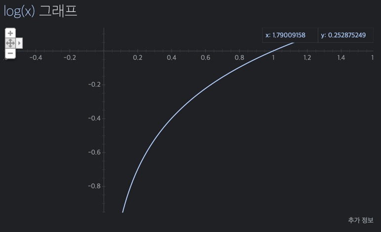
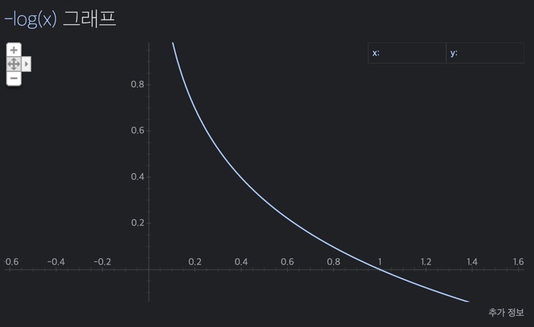
Logarithm function은 위와 같이 단조 증가(monotonically increasing) 함수이기 때문에, 원래 function을 maximizing하는 것은 negative logarithm을 minimizing하는 것과 같다.

위 식의 우변에서 ln에 묶인 항은 \(\mathbf{x}\)와 관련이 없기 때문에 무시할 수 있고, 오른쪽 항을 minimize하게 되면 state에 대한 maximum likelihood estimate를 얻게 된다.

이를 SLAM observation model에 대입하면 다음과 같은 방법으로 해를 얻을 수 있다.

 

\( \begin{align*} \left( \mathbf{x}_k, \mathbf{y}_j \right)^* &= \operatorname{argmax}{\mathcal{N} \left( h (\mathbf{y}_j, \mathbf{x}_k), \mathbf{Q}_{k,j} \right)} \\ &= \operatorname{argmax}{\left( (\mathbf{z}_{k,j} - h (\mathbf{x}_k, \mathbf{y}_j))^T \mathbf{Q}_{k,j}^{-1} (\mathbf{z}_{k,j} - h(\mathbf{x}_k, \mathbf{y}_j)) \right)} \end{align*} \)

 

이 식은 noise term(error)을 minimize하는 2차식이고, 두 번째 식의 2차식은 Mahalanobis distance이다. 즉, information matrix(Gaussian covariance matrix의 역)인 \(\mathbf{Q}_{k,j}^{-1}\)로 weighted된 Euclidean distance(\(\mathcal{L}_2\)-norm)으로 생각할 수 있다.

 

참고로, Mahalanobis distance는 평균과의 떨어진 정도(거리)가 표준편차의 몇 배인지를 나타낸다. 즉, 어떤 값이 얼마나 일어나기 힘든 값인지, 얼마나 이상한 값(outlier)인지를 나타내는 척도이다.

 

 

For all observations

 

이제 모든 observation에 대한 MLE 식을 구해보자. Joint distribution으로 다음과 같이 나타낼 수 있다. (단, input끼리, observation끼리 서로 독립적이고, input과 observation도 서로 독립이다.)

 

\( P \left( \mathbf{z, u} \vert \mathbf{x, y} \right) = \prod\limits_{k} P \left( \mathbf{u}_k \vert \mathbf{x}_{k-1}, \mathbf{x}_k \right) \prod\limits_{k, j} P \left( \mathbf{z}_{k,j} \vert \mathbf{x}_k, \mathbf{y}_j \right) \)

 

모델과 실제 데이터에 대한 error를 다음과 같이 정의하자.

 

\( \mathbf{e}_{u,k} = \mathbf{x}_k - f \left( \mathbf{x}_{k-1}, \mathbf{u}_k \right) \)
\( \mathbf{e}_{z,j,k} = \mathbf{z}_{k,j} - h \left( \mathbf{x}_k, \mathbf{y}_j \right) \)

 

Mahalanobis distance를 최소화하는 것이 결국 MLE를 찾는 것과 같으므로 중간 과정은 이전과 같다. 최종 목표인 \(J\)를 최소화하는 \(\mathbf{x, y}\)를 찾는 식을 아래와 같이 나타낼 수 있다.

 

\( \min{J(\mathbf{x, y})} = \sum\limits_{k} \mathbf{e}_{u,k}^T \mathbf{R}_k^{-1} \mathbf{e}_{u,k} + \sum\limits_{k} \sum\limits_{j} \mathbf{e}_{z,k,j}^T \mathbf{Q}_{k,j}^{-1} \mathbf{e}_{z,k,j} \)

 

이렇게 MLE에서와 같은 해를 least-square problem에서 얻을 수 있게 되었다.

하지만, 노이즈때문에 실제 SLAM 과정에 완벽하게 맞지 않을 것이다. 따라서 state의 추정 값에 대해 fine-tuning을 거친 후 전체적인 error를 감소시킨다. 이 과정이 바로 전형적인 nonlinear optimization 과정이다.

 

 

 

3 Structures of Least-square Problem in SLAM

 

최종 식을 통해, SLAM에서 least-square problem은 다음과 같은 구조를 갖고 있다.

1. State variale의 차원이 아주 높더라도, 각 error term은 하나 또는 두 개의 state variables와만 관련된다. (simple하다.) 이로 인해 SLAM에서는 sparse least-square problem을 얻게 된다.
   • 예를 들어, motion error는 \(\mathbf{x}_{k-1}\)과 \(\mathbf{x}_k\) state variables (2개)에만 관련이 있고, observation error는 \( \mathbf{x}_k, \mathbf{y}_j \) state variables(2개)에만 관련이 있다.
2. 증가량을 표현하는 데 Lie algebra를 사용하면 제한이 없는 optimization problem을, rotation/transformation matrix를 사용하게 되면 제한이 있는 optimization problem을 풀게 된다. 제한이 있는 경우 optimization은 매우 어려워진다.
   • 예를 들어, rotation matrix는 \( \mathbf{R}^T \mathbf{R} = \mathbf{I}, \text{det}(\mathbf{R}) = 1\) 조건을 만족해야 한다.
3. 2차식 metric error, 즉 \(\mathcal{L}_2 \text{-norm}\)을 사용했다. (물론, information matrix가 가중치로 적용된다.)
   • 예를 들어, observation이 아주 정확하다면, covariance matrix는 작고 information matrix는 클 것이며, 이에 따라 해당 error term은 높은 가중치를 갖게 된다. 이후에 \(\mathcal{L}_2\) error의 단점을 살펴볼 것이다.

 

 

 

 

Example: Batch State Estimation

 

이제 예시를 통해 least-square problem을 푸는 방법을 살펴볼 것이다.

아주 간단한 discrete-time system을 예로 들면,

 

\( \begin{cases} x_k = x_{k-1} + u_k + w_k, & \quad \quad w_k \sim \mathcal{N}(0, Q_k) \\ z_k = x_k + n_k, & \quad \quad n_k \sim \mathcal{N}(0, R_k) \end{cases} \)

 

위 식은 앞뒤로(x 축 방향으로) 움직이는 자동차를 나타낸 것이다. 첫 번째 식은 \(u_k\)가 입력, \(w_k\)가 noise인 motion model, 두 번째 식은 \(z_k\)가 측정된 위치인 observation model이다.

\(x_0\)는 주어져있고, time \(k = 1, \cdots, 3\)에 대한 state를 추정해보자.

 

먼저, batch state variable을 \( \mathbf{x} = \left[ x_0, x_1, x_2, x_3 \right]^T \)로, batch observation을 \( \mathbf{z} = \left[ z_1, z_2, z_3 \right]^T \)로 둔다. 또한 \( \mathbf{u} = \left[ u_1, u_2, u_3 \right]^T \)를 정의한다.

이에 따른 MLE는 다음과 같이 구할 수 있다.

 

\( \begin{align*} \mathbf{x}_{map}^* &= \operatorname{argmax}{P(\mathbf{x} \vert \mathbf{u}, \mathbf{z})} = \operatorname{argmax}{P(\mathbf{u, z} \vert \mathbf{x})} \\ &= \prod\limits_{k=1}^3 P(u_k \vert x_{k-1}, x_k) \prod\limits_{k=1}^3 P (z_k \vert x_k) \end{align*} \)

 

다음으로, motion equation과 observation equation에 대해 다음과 같이 식을 변형한다.

 

\( P(u_k \vert x_{k-1}, x_k) = \mathcal{N}(x_k - x_{k-1}, Q_k) \)

\( P(z_k \vert x_k) = \mathcal{N}(x_k, R_k) \)

 

에러는 각각 다음과 같다.

 

\( e_{u,k} = x_k - x_{k-1} - u_k, \quad \quad e_{z,k} = z_k - x_k, \)

 

이에 따라 least-square에 대한 object function은 다음과 같다.

 

\( \min{\sum\limits_{k=1}^{3} e_{u,k}^T Q_k^{-1} e_{u,k} + \sum\limits_{k=1}^{3} e_{z,k}^T R_k^{-1} e_{z,k} } \)

 

Linear system이므로, 수식을 다음과 같이 vector 혹은 matrix 형태로 나타낼 수 있다. 벡터 \(\mathbf{y} = \left[ \mathbf{u, z} \right]^T \)로 정이하면 error는 다음과 같이 정의된다.

 

\( \mathbf{y - Hx} = \mathbf{e} \sim \mathcal{N}(\boldsymbol{0}, \boldsymbol{\Sigma}) \)

 

여기서 \(\mathbf{H}\)는 주어진 식에 따라 다음과 같이 정의된다.

 

\( \mathbf{H} = \begin{bmatrix} 1 & -1 & 0 & 0 \\ 0 & 1 & -1 & 0 \\ 0 & 0 & 1 & -1 \\ \hline 0 & 1 & 0 & 0 \\ 0 & 0 & 1 & 0 \\ 0 & 0 & 0 & 1 \end{bmatrix} \)

 

그리고 \( \boldsymbol{\Sigma} = \text{diag}(Q_1, Q_2, Q_3, R_1, R_2, R_3) \)이다.

따라서 전체 식은 다음과 같이 나타낼 수 있다.

 

\( \mathbf{x}_{map}^* = \operatorname{argmin} \mathbf{e}^T \boldsymbol{\Sigma}^{-1} \mathbf{e} \)

 

이를 풀면 \((\mathbf{H}^T \boldsymbol{\Sigma}^{-1} \mathbf{H})^{-1}\)의 역행렬이 존재하기 때문에 다음과 같은 유일해를 갖는다. (풀이 과정은 나중에 알아볼 것이다.)

 

\( \mathbf{x}_{map}^* = \left( \mathbf{H}^T \boldsymbol{\Sigma}^{-1} \mathbf{H} \right)^{-1} \mathbf{H}^T \boldsymbol{\Sigma}^{-1} \mathbf{y} \)

 

 

다음 포스팅에서는 본격적으로 least-square problem을 어떻게 푸는지 Gauss-Newton method, Levernberg-Marquatdt method 등을 포함하여 알아볼 것이다.