Lie Group and Lie Algebra (1) - 정의, so(3), se(3), Exponential Mapping, Logarithmic Mapping

Xiang Gao, Tao Zhang 저자의 'Introduction to Visual SLAM from Theory to Practice' 책을 통해 SLAM에 대해 공부한 내용을 기록하고자 한다.

책의 내용은 주로 'SLAM의 기초 이론', 'system architecture', 'mainstream module'을 다룬다.

 

포스팅에는 기초 이론만 다룰 것이며, 실습을 해보고 싶다면 다음 github를 참조하자.

 

https://github.com/gaoxiang12/slambook2

GitHub - gaoxiang12/slambook2: edition 2 of the slambook

 

 

목차

 

 

 

 

이전까지 3차원 공간 상에서 강체의 motion에 대해 알아보았다.

특히 motion의 표현에 대해 집중적으로 알아보았는데, 사실 SLAM에서는 motion의 표현에서 더 나아가 estimate(추정)와 optimize(최적화)를 해야한다.

SLAM에서 pose는 알 수 없기 때문에, 어떤 카메라 포즈가 현재 관측 결과와 가장 잘 맞는지에 대한 문제를 해결해야 한다. 이때 일반적으로 optimization problem을 정의하고, 최적의 \(\boldsymbol{R}, \boldsymbol{t}\) 해를 구하고 error를 최소화한다.

 

이전 포스팅에서 설명했듯, rotation matrix는 제한적인 matrix이다. (orthogonal이며, determinant 값이 1이어야 함)

따라서 rotation matrix를 optimization variable로 사용하게 되면 추가적인 제한이 생겨 최적화 과정이 더 어려워진다.

이때 transformation relationship을 Lie group과 Lie algebra를 사용하여 나타내면 pose estimation을 (제한 없는)optimization problem으로 바꿀 수 있다.

내용이 아주 복잡하고 어렵지만, 기초적인 Lie group과 Lie algebra 내용을 살펴보자.

 

 

 

 

 

 Basics of Lie Group and Lie Algebra

 

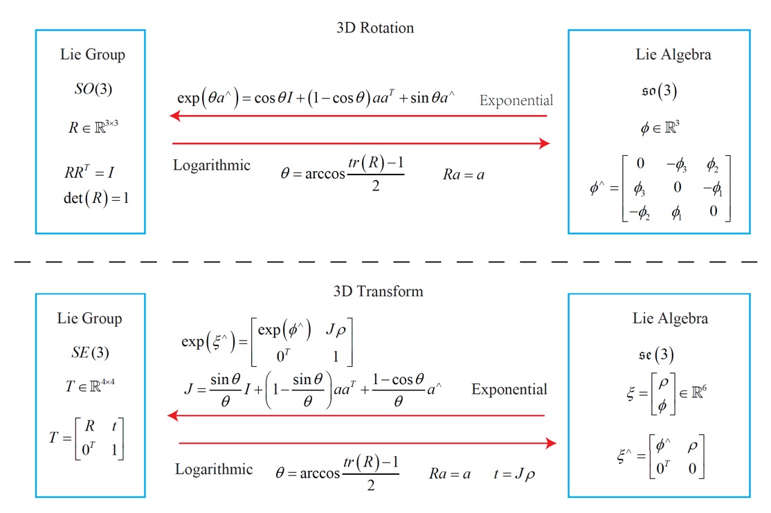
Rotation matrix를 설명하면서, 3차원 rotation matrix의 경우 special orthogonal group \(\text{SO}(3)\)를, transformation matrix는 \(\text{SE}(3)\)를 구성한다고 하였다.

이를 수식으로 표현하면 다음과 같다.

 

\( \text{SO}(3) = \left\{ \boldsymbol{R} \in \mathbb{R}^{3 \times 3} \vert \boldsymbol{R} \boldsymbol{R}^T = \boldsymbol{I}, \text{det}(\boldsymbol{R}) = 1 \right\} \)
\( \text{SE}(3) = \left\{ \boldsymbol{T} = \begin{bmatrix} \boldsymbol{R} & \boldsymbol{t} \\ \boldsymbol{0}^T & 1 \end{bmatrix} \in \mathbb{R}^{4 \times 4} \vert \boldsymbol{R} \in \text{SO}(3), \boldsymbol{t} \in \mathbb{R}^3 \right\} \)

 

그리고 rotation matrix와 transformation matrix 둘 다 연속된 rotation 또는 transformation을 곱셈으로 표현하였지, 덧셈에 관해서는 언급하지 않았다.

그 이유는, \(\text{SO}, \text{SE}\) group이 모두 addition에 대해서는 닫혀있지 않기 때문이다.

 

\( \boldsymbol{R}_1 + \boldsymbol{R}_2 \notin \text{SO}(3), \quad \quad \boldsymbol{T}_1 + \boldsymbol{T}_2 \notin \text{SE}(3) \)

 

곱셈 연산에 대해서만 다음과 같이 닫혀있다.

 

\( \boldsymbol{R}_1 \boldsymbol{R}_2 \in \text{SO}(3), \quad \quad \boldsymbol{T}_1 \boldsymbol{T}_2 \in \text{SE}(3) \)

 

이와 같이 하나의 연산에만 "well-defined"되는 집합을 group이라 한다.

 

 

 

 

 Group

 

Group의 기본적인 개념을 살펴보자.

Group은 하나의 집합(set)과 하나의 연산(operator)으로 이루어진 대수적인 구조(algebraic structure)이다.

만약 어떤 group을 이루는 집합 \(A\)와 연산 \(\cdot\)이 있다면, 이 group은 다음과 같이 표현한다.

 

\( G = (A, \cdot) \)

 

이때 \(G\)가 group이 되기 위해서는 다음과 같은 조건을 만족해야 한다.

 

1. Closure (닫혀 있음) : \( \forall a_1, a_2 \in A, a_1 \cdot a_2 \in A  \)
2. Combination (결합 법칙) : \( \forall a_1, a_2, a_3 \in A, (a_1 \cdot a_2) \cdot a_3 = a_1 \cdot (a_2 \cdot a_3) \)
3. Unit element (항등원) : \( \exists a_0 \in A, \text{s.t.} \forall a \in A, a_0 \cdot a = a \cdot a_0 = a \)
4. Inverse element (역원) : \( \forall a \in A, \exists a^{-1} \in A, \text{s.t.} a \cdot a^{-1} = a_0 \)

 

간단히 설명하자면, 집합 \(A\)의 모든 요소에 대해 \(\cdot\) 연산에 대해 닫혀있어야 하고(1), 연산에 대한 결합 법칙을 만족하며(2), 각 값에 대한 항등원(3)과 역원(4)이 존재해야 한다.

 

group의 간단한 예를 들자면, 앞서 설명한 (rotation matrix, matrix multiplication), (transformation matrix, matrix multiplication), addition of integers ( \( ( \mathbb{Z}, + ) \) ), 0을 제외한 rational number(유리수)과 multiplication ( \( (\mathbb{Q} \backslash 0, \cdot ) \) ) 등이 있다.

 

행렬에서의 일반적인 group은 다음과 같다.

• General Linear group \( \text{GL}(n)\)
  • Invertiable n by n matrix와 matrix multiplication
• Special Orthogonal group (rotation matrix group) \( \text{SO}(n)\)
• Special Euclidean group (n dimensional transformation) \( \text{SE}(n)\)

 

Group 개념은 group의 연산이 아주 좋은 특성을 갖는다는 것을 보여준다.

 

Lie Group은 연속적인 (continuous, smooth) 특성을 갖는 group을 말한다. Integer group \( \mathbb{Z} \) 등은 불연속이므로 Lie Group이 될 수 없다.

그리고, \(\text{SO}(n), \text{SE}(n)\)의 경우에는 강체는 당연히 실 세계에서 연속적으로 움직이기 때문에 직관적으로 real space에서 연속임을 알 수 있다.

Camera의 자세 추정 (pose estimation)에서 \( \text{SO}(n), \text{SE}(3) \)이 특히 중요하기 때문에, 이 두 개의 Lie group에 대해 알아볼 것이다.

 

연속적이라는 것을 엄밀히 판단하기 위해서는 analysis와 topology의 개념이 필요하다. 이를 위해서는 수학적으로 깊은 지식이 필요한데, 이 책의 내용이 수학을 main으로 다루는 것은 아니므로 SLAM과 관련된 중요한 부분만 다루도록 한다.

 

 

 

 

 Introduction of the Lie Algebra

 

어떤 rotation matrix \( \boldsymbol{R} \)이 시간 \(t\)에 따라 연속적으로 회전하는 카메라의 회전을 나타내는 함수로 표현된다면 다음을 만족할 것이다.

 

\( \boldsymbol{R}(t) \boldsymbol{R}(t)^T = \boldsymbol{I} \)

 

양변을 시간 \(t\)에 대해 미분하고 정리하면

 

\( \dot{\boldsymbol{R}}(t) \boldsymbol{R}(t)^T + \boldsymbol{R}(t) \dot{\boldsymbol{R}}(t)^T = 0 \)

\( \dot{\boldsymbol{R}}(t) \boldsymbol{R}(t)^T = - \left( \dot{\boldsymbol{R}}(t) \boldsymbol{R}(t)^T \right)^T \)

 

마지막 식을 보면 \( \dot{\boldsymbol{R}}(t) \boldsymbol{R}(t)^T \) term이 skew-symmetric matrix임을 알 수 있다.

cross product 식을 나타내는 '\( ^\wedge \)' symbol을 활용하여 vector를 skew-symmetric matrix로 나타냈듯이, 어떤 skew-symmetric matrix에 해당하는 유일한 vector를 다음과 같이 나타낼 수 있다.

 

\( \mathbf{a^\wedge = A = } \begin{bmatrix} 0 & -a_3 & a_2 \\ a_3 & 0 & -a_1 \\ -a_2 & a_1 & 0 \end{bmatrix}, \quad \mathbf{A^\vee = a} \)

 

이에 따라 \( \mathbf{\dot{R}}(t) \mathbf{R}(t)^T \)는 skey-symmetric matrix이므로 이에 해당하는 3차원 벡터 \( \boldsymbol{\phi}(t) \in \mathbb{R}^3 \)를 사용하여 다음과 같이 정의할 수 있다.

 

\( \dot{\mathbf{R}}(t) \mathbf{R}(t)^T = \boldsymbol{\phi}(t)^\wedge \)

 

여기서 \( \mathbf{R}(t) \)를 양 변에 곱하면 다음과 같이 식을 변형할 수 있다.

 

\( \dot{\mathbf{R}}(t) = \boldsymbol{\phi}(t)^\wedge \mathbf{R}(t) = \begin{bmatrix} 0 & - \phi_3 & \phi_2 \\ \phi_3 & 0 & -\phi_1 \\ -\phi_2 & \phi_1 & 0 \end{bmatrix} \mathbf{R}(t) \)

 

식의 형태를 살펴보면, rotation matrix \( \mathbf{R}(t) \) 왼쪽에 \( \boldsymbol{\phi}^\wedge (t) \) matrix를 곱하는 것으로 rotation matrix의 도함수를 구할 수 있다는 것을 알 수 있다.

 

초기 시간 \(t_0 = 0 \)이라 하면, \(\boldsymbol{\phi}(t_0) = \boldsymbol{\phi}_0 \)이므로, initial value \( \mathbf{R}(0) = \mathbf{I} \)에 따른 미분 방정식의 해를 구하는 과정과 결과는 다음과 같다.

 

미분방정식 풀이 과정

 

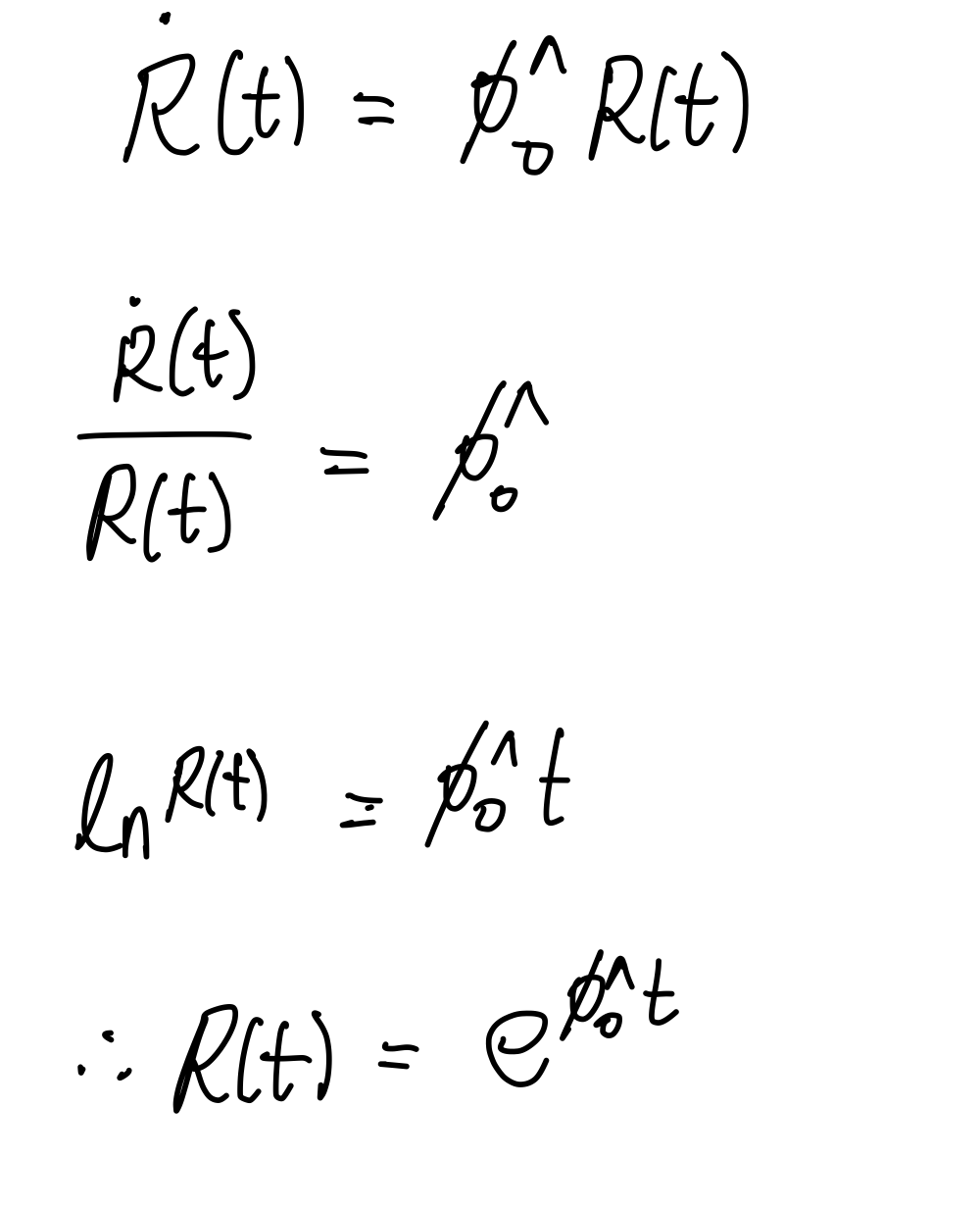
\( \mathbf{R}(t) = \text{exp} \left( \boldsymbol{\phi}_0^\wedge t \right) \)

 

또한, 초기 시간 \(t_0 = 0\)일 때 rotation matrix \( \mathbf{R}(0) = \mathbf{I} \)임을 고려해보면, 도함수의 식과 \(t\)가 \(t_0\) 근처일 때의 first-order Taylor expansion에 따라 \( \mathbf{R}(t) \)를 다음과 같이 나타낼 수 있다.

 

\( \mathbf{R}(t) \approx \mathbf{R}(t_0) + \dot{\mathbf{R}}(t_0) (t - t_0) = \mathbf{I} + \boldsymbol{\phi}(t_0)^\wedge (t) \)

 

그리고 여기서 \( \boldsymbol{\phi} \)는 \( \mathbf{R} \)의 도함수를 나타내므로, \( \text{SO}(3) \)의 origin 근처에서의 tangent space라 불린다.

 

다시 미분방정식의 해로 돌아가서, 해당 식은 \(t\)가 0 근처일 때의 rotation matrix는 \( \boldsymbol{\phi}_0^\wedge t \)라는 행렬에 exponential을 취하여 계산할 수 있다는 것, 즉 rotation matrix \( \mathbf{R}\)은 또다른 skew-symmetric matrix \( \boldsymbol{\phi}_0^\wedge t \)와 exponential 관계를 갖는다는 것을 뜻한다.

하지만 matrix의 exponenetial은 무엇인지에 대한 대답을 위해서는 다음을 명확히 해야 한다.

1. 특정 순간에 \( \mathbf{R}\)이 주어졌을 때, \( \mathbf{R} \)의 local derivate 관계를 설명하는 \( \boldsymbol{\phi} \)를 찾을 수 있다. 이들이 서로 어떤 관련이 있는가?
   • 이 개념을 "\( \boldsymbol{\phi}\)는 \( \text{SO}(3) \) 상에서 Lie Algebra인 \( \mathfrak{so}(3) \)에 상응한다."라고 말할 것이다.
2. vector \( \boldsymbol{\phi} \)가 주어졌을 때, \( \text{exp} \left( \boldsymbol{\phi}^\wedge \right) \)를 어떻게 구할 것인가? 역으로, \( \mathbf{R} \)이 주어졌을 때 \( \boldsymbol{\phi} \)를 구하기 위한 반대 연산이 존재하는가?
   • 이는 Lie group과 Lie algebra 사이의 Exponential/logarithmic mapping을 통해 이루어진다.

 

이 두 가지 문제를 해결해보자.

 

 

 

 

 Definition of Lie Algebra

 

각 Lie group은 그에 상응하는 Lie Algebra를 갖는다.

Lie Algebra는 origin point 근처에서 Lie group의 local structure(tangent space)를 묘사한다.

Lie Algebra의 일반적인 정의는 다음과 같다.

 

집합 \( \mathbb{V} \), scalar field \( \mathbb{F} \), binary operation \( [,] \)으로 이루어진 Lie algebra에 대해, 다음과 같은 성질을 만족한다면 \( \left( \mathbb{V, F, [,] } \right) \)는 Lie algebra이며, \( \mathfrak{g} \)로 나타낸다.
1. Closure ([,] 연산에 대해 닫혀있음) : \( \forall \mathbf{X, Y} \in \mathbb{V}; \left[ \mathbf{X, Y} \right] \in \mathbb{V} \)
2. Bilinear composition (이중 선형 결합) : \( \forall \mathbf{X, Y, Z} \in \mathbb{V}; a, b \in \mathbb{F},  \)이면
$$ \left[ a \mathbf{X} + b \mathbf{Y}, \mathbf{Z} \right] = a \left[ \mathbf{X, Z} \right] + b \left[ \mathbf{Y, Z} \right], \quad \left[ \mathbf{Z}, a \mathbf{X} + b \mathbf{Y} \right] = a \left[ \mathbf{Z, X} \right] + b \left[ \mathbf{Z, Y} \right] $$
3. Reflexive : \( \forall \mathbf{X} \in \mathbb{V}; \left[ \mathbf{X, X} \right] = \boldsymbol{0} \)
4. Jacobi identity : \( \forall \mathbf{X, Y, Z} \in \mathbb{V}; \mathbf{ \left[ X, \left[ Y, Z \right] \right] + \left[ Z, \left[ X, Y \right] \right] + \left[ Y, \left[Z, X \right] \right] = 0} \)

 

여기서 binary ooperation인 \( [,] \)는 Lie bracket이라 한다. 이 연산은 group 내에서의 다른 (더 간단한) 이진 연산들에 비해 두 elements 간의 difference를 표현해준다.

결합법칙은 만족할 필요가 없으나, 'Reflexive' 성질과 같이 같은 element끼리 연산을 하면 \( \boldsymbol{0} \) 이 되어야 한다.

예를 들어, 3차원 벡터 \(\mathbb{R}^3\)에 대한 cross product인 \( \times\)도 Lie bracket 중 하나이다. 따라서 \( \mathfrak{g} = \left( \mathbb{R}^3, \mathbb{R}, \times \right) \)는 Lie algebra를 구성한다.

 

 

 

 

 Lie Algebra \( \mathfrak{so}(3) \)

 

위에서 언급했던 \( \boldsymbol{\phi}\)는 Lie algebra의 한 종류이다. 즉, \( \text{SO}(3) \)에 상응하는 Lie algebra는 \( \mathbb{R}^3 \)에서 정의된 벡터이고, 이를 \( \boldsymbol{\phi} \)로 나타낸다.

위에서 벡터 \( \boldsymbol{\phi}^\wedge \)로 나타냈던 skew-symmetric matrix를 다음과 같이 나타내기로 하자.

 

\( \boldsymbol{\Phi} = \boldsymbol{\phi}^\wedge = \begin{bmatrix} 0 & - \phi_3 \phi_2 \\ \phi_3 & 0 & -\phi_1 \\ -\phi_2 & \phi_1 & 0 \end{bmatrix} \in \mathbb{R}^{3 \times 3} \)

 

이에 따라 두 벡터 \( \boldsymbol{\phi_1, \phi_2} \)의 Lie bracket은 다음과 같다.

 

\( \left[ \boldsymbol{\phi_1, \phi_2} \right] = \left( \boldsymbol{\Phi_1 \Phi_2 - \Phi_2 \Phi_1} \right)^\vee \)

 

벡터 \( \boldsymbol{\phi}\)와 skew-symmetric matrix는 1:1 대응이므로, \( \mathfrak{so}(3) \)의 element들은 3차원 벡터 또는 3차원 skew-symmetric matrix일 것이다.

 

\( \mathfrak{so}(3) = \left\{ \boldsymbol{\phi} \in \mathbb{R}^3 or \boldsymbol{\Phi = \phi^\wedge} \in \mathbb{R}^{3 \times 3} \right\} \)

 

\( \mathfrak{so}(3) \)의 구성 요소는 rotation matrix의 derivative를 표현하는 3차원 벡터라는 것으로 명확해졌다.

\( \text{SO}(3) \)로의 관계는 앞서 알아보았듯이 exponential mapping으로 주어진다.

Exponential map에 대해서는 조금 후에 알아보고, Lie algebra가 \( \text{SE}(3) \)에 어떻게 대응되는지부터 알아보자.

 

 

 

 

 Lie Algebra \( \mathfrak{se}(3) \)

 

\( \text{SE}(3) \)에 대해서도 상응하는 Lie algebra인 \( \mathfrak{se}(3) \)이 존재한다.

\( \mathfrak{so}(3)\)에서와 비슷하게, \( \mathfrak{se}(3) \)는 \( \mathbb{R}^6 \)공간에 존재한다.

 

\( \mathfrak{se}(3) = \left\{ \boldsymbol{\xi} = \begin{bmatrix} \boldsymbol{\rho} \\ \boldsymbol{\phi} \end{bmatrix} \in \mathbb{R}^6, \boldsymbol{\rho} \in \mathbb{R}^3, \boldsymbol{\phi} \in \mathfrak{so}(3), \boldsymbol{\xi}^\wedge = \begin{bmatrix} \boldsymbol{\phi}^\wedge & \boldsymbol{\rho} \\ \boldsymbol{0}^T & 0 \end{bmatrix} \in \mathbb{R}^{4 \times 4} \right\} \)

 

\( \mathfrak{se}(3) \)의 element를 6차원 벡터인 \( \boldsymbol{\xi} \)로 쓴다.

첫 번째 세 개 차원은 translation 부분 (\( \boldsymbol{\rho} \))이고, 두 번째 세 개 차원은 앞서 계속 언급했던 rotation 부분 (\( \boldsymbol{\phi}\))이다. 이때 translation 부분이라고 해서 matrix에서의 translation과는 다르다는 것에 유의하자.

그리고 \( ^\wedge \) symbol의 이미를 확장하여 \( \mathfrak{se}(3) \)에서는 6차원 벡터가 4차원 matrix로 변환되는 것을 의미하게 된다. (이제 더 이상 결과가 skew-symmetric matrix는 아니다.)

즉, \( ^\wedge, ^\vee \) symbol은 여전히 "vector에서 matrix로의 변환", "matrix에서 vector로의 변환"을 뜻하며, 여전히 일대일 대응이다.

 

한마디로 \( \mathfrak{se}(3) \)는 "\( \mathfrak{so}(3) \) 요소에 translation 부분의 벡터가 추가된 벡터"로 생각할 수 있다.

 

그리고 \( \mathfrak{se}(3) \)또한 다음과 같이 Lie bracket 연산을 갖는다.

 

\( \left[ \boldsymbol{\xi_1, \xi_2} \right] = \left( \boldsymbol{\xi_1^\wedge \xi_2^\wedge - \xi_2^\wedge \xi_1^\wedge} \right)^\vee \)

 

 

 

 

 

 

 Exponential and Logarithmic Mapping

 

'Introduction of Lie Algebra'에서 언급했던 첫 번째 문제는 해결하였다. 이제 두 번째 문제인 즉 exponential/logarithmic mapping을 통한 Lie group과 Lie algebra 사이의 변환을 알아보자.

 

위에서와 마찬가지로, 먼저 \( \mathfrak{so}(3) \)의 mapping을 알아본 후에 \( \mathfrak{se}(3) \)의 경우를 알아보자.

 

 

 

 Exponential & Logarithmic Map of \(\mathfrak{so}(3)\) & \(\text{SO}(3)\)

 

임의의 행렬에 대한 exponential은 Talyer expansion으로 나타낼 수 있다.

 

\( \text{exp} \left( \boldsymbol{\phi}^\wedge \right) = \sum \limits_{n=0}^\infty \frac{1}{n!} \left( \boldsymbol{\phi}^\wedge \right)^n \)

 

exponential mapping을 계산할 때 무한급수를 사용할 수는 없으므로, 형태를 변환해 주어야 한다.

\(\boldsymbol{\phi} \)는 3차원 벡터이므로, length \(\theta\)와 direction \(\mathbf{n}\)으로 아래와 같이 정의해줄 수 있다.

 

\( \boldsymbol{\phi} = \theta \mathbf{n} \)

 

이때 \( \mathbf{n} \)은 단위 방향벡터(\( \lVert \mathbf{n} \rVert \))이다.

이러한 단위방향벡터는 두 가지 성질을 갖는다.

 

\( \mathbf{n}^\wedge \mathbf{n}^\wedge = \begin{bmatrix} -n_2^2 -n_3^2 & n_1 n_2 & n_1 n_3 \\ n_1 n_2 & -n_1^2 - n_3^2 & n_2 n_3 \\ n_1 n_3 & n_2 n_3 & -n_1^2 -n_2^2 \end{bmatrix} = \mathbf{nn}^T - \mathbf{I} \)
\( \mathbf{n}^\wedge \mathbf{n}^\wedge \mathbf{n}^\wedge = \mathbf{n}^\wedge (\mathbf{nn}^T - \mathbf{I} ) = \mathbf{n}^\wedge \mathbf{nn}^T - \mathbf{n}^\wedge = - \mathbf{n}^\wedge \)

 

두 번째 식에서 \( \mathbf{n}^\wedge \mathbf{n} = \boldsymbol{0} \)이므로 최종 결과가 간단하게 나왔다.

 

위 두 식은 고차원의 \( \mathbf{n}^\wedge \) 항을 다루는 방법을 제공해준다. 이를 이용하여 exponential map을 다음과 같이 나타낸다.

 

\( \begin{align*} \text{exp} \left( \boldsymbol{\phi}^\wedge \right) &= \text{exp} \left( \theta \mathbf{n}^\wedge \right) = \sum \limits_{n=0}^{\infty} \frac{1}{n!} \left( \theta \mathbf{n}^\wedge \right)^n \\ &= \mathbf{I + \theta n^\wedge} + \frac{1}{2!} \theta^2 \mathbf{ \mathbf{n}^\wedge \mathbf{n}^\wedge} + \frac{1}{3!} \theta^3 \mathbf{\mathbf{n}^\wedge \mathbf{n}^\wedge \mathbf{n}^\wedge} + \frac{1}{4!} \theta^4 \left( \mathbf{n}^\wedge \right)^4 + \dots \\ &= \mathbf{n}\mathbf{n}^T - \mathbf{n}^\wedge \mathbf{n}^\wedge + \theta \mathbf{n}^\wedge + \frac{1}{2!} \theta^2 \mathbf{n}^\wedge \mathbf{n}^\wedge - \frac{1}{3!} \theta^3 \mathbf{n}^\wedge - \frac{1}{4!} \theta^4 \left( \mathbf{n}^\wedge \right)^2 + \dots \\ &= \mathbf{n} \mathbf{n}^T + \left( \theta - \frac{1}{3!} \theta^3 + \frac{1}{5!} \theta^5 - \dots \right) \mathbf{n}^\wedge - \left( 1 - \frac{1}{2!} \theta^2 + \frac{1}{4!} \theta^4 - \dots \right) \mathbf{n}^\wedge \mathbf{n}^\wedge \\ &= \mathbf{n}^\wedge \mathbf{n}^\wedge + \mathbf{I} + \sin{\theta} \mathbf{n}^\wedge - \cos{\theta} \mathbf{n}^\wedge \mathbf{n}^\wedge \\ &= (1 - \cos{\theta}) \mathbf{n}^\wedge \mathbf{n}^\wedge + \mathbf{I} + \sin{\theta} \mathbf{n}^\wedge \\ &= \cos{\theta} \mathbf{I} + (1 - \cos{\theta}) \mathbf{nn}^T + \sin{\theta} \mathbf{n}^\wedge \end{align*} \)

 

최종적으로 다음 식을 얻게 된다.

 

\( \text{exp} \left( \theta \mathbf{n}^\wedge \right) = \cos{\theta} \mathbf{I} + (1 - \cos{\theta}) \mathbf{nn}^T + \sin{\theta} \mathbf{n}^\wedge \)

 

"3D Rigid Body Motion" 포스팅에서 알아보았던 Rodrigues' formula와 같다는 것을 알 수 있다.

이는 곧 \( \mathfrak{so}(3) \)는 rotation vector, exponential map은 Rodrigues' formula임을 보여준다.

 

이러한 exponential map을 통해 \( \mathfrak{so}(3) \)의 벡터를 \( \text{SO}(3) \)의 rotation matrix로 mapping할 수 있고, 역으로 logarithmic map을 통해 \( \text{SO}(3)\)의 요소를 \( \mathfrak{so}(3) \)로 mapping 가능하다.

 

 

 

 

 Exponential & Logarithmic Map of \(\mathfrak{se}(3)\) & \(\text{SE}(3)\)

 

\( \mathfrak{se}(3) \)의 mapping의 개념은 비슷하다. 단지 \( \boldsymbol{\phi} \) 벡터를 \( \boldsymbol{\xi} \)로 확장했을 뿐이다.

한 가지 주목할 점은 Taylor expansion을 적용할 때 아래와 같이 upper left의 3 × 3 matrix, upper right의 3 × 1 vector, lower left의 1 × 3 vector, lower right의 scalar로 4가지 부분으로 나뉘어 적용된다는 점이다.

 

\( \text{exp} \left( \xi^\wedge \right) = \begin{bmatrix} \sum \limits_{n=0}^{\infty} \frac{1}{n!} \left( \boldsymbol{\phi}^\wedge \right)^n & \sum \limits_{n=0}^{\infty} \frac{1}{(n+1)!} \left( \boldsymbol{\phi}^\wedge \right)^n \boldsymbol{\rho} \\ \boldsymbol{0}^T & 1 \end{bmatrix} \triangleq \begin{bmatrix} \mathbf{R} & \mathbf{J} \rho \\ \boldsymbol{0}^T & 1 \end{bmatrix} = \mathbf{T} \)

 

이후의 증명 로직은 \(\mathfrak{so}(3)\)에서와 같으므로 생략한다.

Taylor expansion을 적용할 때 다음과 같이 \( \mathbf{J} \) 부분이 조금 달라지게 된다.

 

\( \mathbf{J} = \frac{\sin{\theta}}{\theta} \mathbf{I} + \left( 1 - \frac{\sin{\theta}}{\theta} \right) \mathbf{aa}^T + \frac{1 - \cos{\theta}}{\theta} \mathbf{a}^\wedge \)

 

위 식은 어느 정도 Rodrigues formula와 비슷한 형태이지만, 완전히 같지는 않다.

식을 살펴보면 exponential mapping 이후 translation 부분이 linear jacobian matrix \( \mathbf{J} \)와 곱해졌다.

이 jacobian matrix는 나중에 활용될 것이므로 기억해두자.

 

비슷한 방법으로 logarithmic mapping을 유도할 수 있는데, transformation matrix \( \mathbf{T} \)에 따라 좀 더 쉬운 방법으로 대응하는 벡터인 \( \mathfrak{so}(3) \)를 찾을 수 있다.

Transformation matrix \( \mathbf{T} \)는 upper left corner에 rotation matrix \( \mathbf{R} \)을 포함하고, upper right corner에 translation vector \( \mathbf{t} \)를 포함하며, 다음을 만족한다.

 

\( \mathbf{t = J} \boldsymbol{\rho} \)

 

\( \mathbf{J} \)를 \( \boldsymbol{\phi} \)로부터 얻을 수 있기 때문에, \( \boldsymbol{\rho} \) 또한 위 식과 같은 linear equation으로 얻을 수 있다.

 

 

 

 

 Summary

 

Lie group과 Lie algebra의 상호 변환 관계를 다음과 같이 요약해볼 수 있다.

 

Mutual Conversion Relationship

 

다음 포스팅은 이어서 'Lie Algebra Derivation and Perturbation Model'에 대해 알아볼 것이다.

좀 더 복잡한 내용이니, 이번 포스팅 내용을 잘 숙지해두자.