목차
Flow-based Models (1)에서 모델을 전반적으로 이해해보았다. 본 포스팅에서는 flow-based model의 예시를 알아보자.
Flow-based model은 invertible transformation에 어떤 함수를 사용하는지에 따라 나뉜다.
Planar Flows
Planar flow에서의 invertible transformation은 다음과 같다. (편의 상 bold체를 따로 사용하지 않고 벡터를 표현한다.)
\( x = f_\theta (z) = z + u h (w^\top z + b) \)
위 식과 같이 \(\theta = (w, u, b)\)로 parameterize하고, non-linearity \(h(\cdot)\)이 non-linearity라 할 때, Jacobian의 determinant의 절댓값은 다음과 같이 구할 수 있다.
\( \begin{align*} \left\vert \operatorname{dete} \left( \cfrac{\partial f_\theta (z)}{\partial z} \right) \right\vert &= \left\vert \operatorname{det} (I + h'(w^\top z + b) u w^\top ) \right\vert \\ &= \left\vert 1 + h'(w^\top z + b) u^\top w \right\vert \end{align*} \)
그런데, invertible 성질을 만족하기 위해서는 다음과 같은 두 가지 제약조건이 필요하다.
\( h = \operatorname{tanh} (\cdot) \)
\( h' (w^\top z + b) u^\top w \geq -1 \)
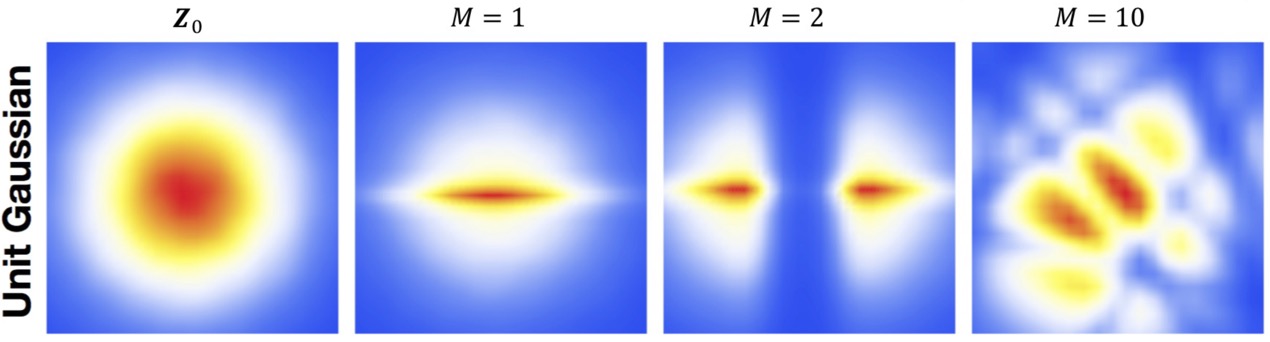
Base distribution \(\pi\)가 Gaussian distribution인 경우와 Uniform distribution인 경우, M개 (이전 글에서의 \(K\)) transformation 후 distribution을 시각화해보면 다음과 같은 결과를 보인다.

NICE and Real-NVP
NICE와 Real-NVP라는 flow-based model을 알아보자. 특히 Real-NVP는 GLOW 등 좋은 성능을 보이는 다른 flow-based model들의 기본이 되는 중요한 모델이다.
Nonlinear Independent Components Estimation (NICE)
NICE는 additive coupling layer와 rescaling layer 이렇게 두 가지 invertible transformation으로 구성된다.
Additive coupling layers
Additive coupling layer에서는 random variable \(\mathbf{z}\)를 두 subset \(\mathbf{z}_{1:d}\)와 \(\mathbf{z}_{d+1:D}\)으로 나눈다. 이때 \(1 \leq d < D\)는 랜덤으로 고른다.
그리고 layer에서는 두 가지 연산 forward mapping \( \mathbf{z} \mapsto \mathbf{x} \)와 inverse mapping \( \mathbf{x} \mapsto \mathbf{z} \)을 수행한다.
먼저 forward mapping은 아래와 같이 진행된다.
\( \mathbf{x}_{1:d} = \mathbf{z}_{1:d} \quad \text{identity transformation} \)
\( \mathbf{x}_{d+1:D} = \mathbf{z}_{d+1:D} - \mathcal{M}_{\boldsymbol{\theta}} (\mathbf{z}_{1:d}) \)
- \(\mathcal{M}_{\boldsymbol{\theta}}\) : \(d\)개 input units, \(D-d\)개 output units를 갖는 neural network
첫 번째 subset에 대해서는 identity transformation(그대로 transform), 두 번째 subset에 대해서는 첫 번째 subset을 입력한 neural network의 결과를 뺀 결과를 \(x\)로 맵핑하는 transformation이다.
이때 Jacobian은 다음과 같이 계산한다.
\( \mathbf{J} = \cfrac{\partial \mathbf{x}}{\partial \mathbf{z}} = \begin{bmatrix} \mathbf{I}_{d \times d} & \boldsymbol{0}_{d \times (D-d)} \\ \cfrac{\partial \mathbf{x}_{d+1:D}}{\partial \mathbf{z}_{1:d}} & \mathbf{I}_{(D-d) \times (D-d)} \end{bmatrix} \)
Jacobian은 lower triangular matrix 형태로 나오며, determinant가 1이므로 volume이 보존된다. (volume preserving transformation)
또한 inverse mapping은 아래와 같이 진행한다.
\( \mathbf{z}_{1:d} = \mathbf{x}_{1:d} \quad \text{identity transformation} \)
\( \mathbf{z}_{d+1:D} = \mathbf{x}_{d+1:D} + \mathcal{M}_{\boldsymbol{\theta}} (\mathbf{x_{1:d}}) \)
Forward mapping에서 사용했던 neural network를 그대로 활용하여 \(\mathbf{x}\)를 \(\mathbf{z}\)로 맵핑한다.
NICE에서는 여러 개의 서로 다른 \(d\)값을 갖는, 즉 partition이 서로 다른 additive coupling layer들을 거친다.
Rescaling layeres
Rescaling layer는 여러 additive coupling layer를 거친 후 마지막 layer에서 동작하는 transformation이다.
마찬가지로 forward mapping \( \mathbf{z} \mapsto \mathbf{x} \)와 inverse mapping \( \mathbf{x} \mapsto \mathbf{z} \)을 수행한다.
Forward mapping부터 살펴보자.
\( x_i = s_i z_i \)
- \(s_i\) : \(i\)번째 dimension에 대한 scaling factor
즉, 단순히 \(\mathbf{z}\)의 요소 각각에 scaling factor를 곱해주는 과정이다.
Jacobian도 간단하다.
\( \mathbf{J} = \operatorname{diag} (s) \)
\( \operatorname{det} (\mathbf{J}) = \prod\limits_{i=1}^D s_i \)
Inverse mapping은 자연스럽게 다음과 같이 계산한다.
\( z_i = \cfrac{x_i}{s_i} \)
Real-valued Non-volume Preserving Flows (Real-NVP)
Real-NVP도 NICE와 비슷하게 coupling layer와 permutation layer 두 가지 layer로 구성된다. 단, 이름에서 알 수 있듯이, Jacobian의 determinant가 1이 아닌, non-volume preserving transformation을 활용한다.
Coupling layers
NICE에서의 additive coupling layer와 마찬가지로, 우선 variable \(\mathbf{z}\)를 두 subset \(\mathbf{z}_{1:d}\)와 \(\mathbf{z}_{d+1:D}\)으로 나눈다. (마찬가지로 \(1 \leq d < D\))
Forward mapping \(\mathbf{z} \mapsto \mathbf{x}\)는 다음과 같다.
\( \mathbf{x}_{1:d} = \mathbf{z}_{1:d} \quad \text{identity transformation} \)
\( \mathbf{x}_{d+1:D} = \mathbf{z}_{d+1:D} \odot \operatorname{exp} \left( s (\mathbf{z}_{1:d}) \right) + t \left( \mathbf{z}_{1:d} \right) \)
- \(s(\cdot)\), \(t(\cdot)\) : 각각 scaling, transition neural network로, \(d\)개 units을 입력받아 \(n-d\)개 units를 출력한다.
- \(\odot\) : Element-wise 곱(production)을 나타낸다.
Inverse mapping \(\mathbf{x} \mapsto \mathbf{z}\)는 다음과 같다.
\( \mathbf{z}_{1:d} = \mathbf{x}_{1:d} \quad \text{identity transformation} \)
\( \mathbf{z}_{d+1:D} = \left( \mathbf{x}_{d+1:D} - t ( \mathbf{x}_{1:d} ) \right) \odot \operatorname{exp} \left( - s ( \mathbf{x}_{1:d} ) \right) \)
Jacobian과 그 determinant는 다음과 같이 계산한다.
\( \mathbf{J} = \cfrac{\partial \mathbf{x}}{\partial \mathbf{z}} = \begin{bmatrix} \mathbf{I}_{d \times d} & \boldsymbol{0}_{d \times (D - d)} \\ \cfrac{\partial \mathbf{x}_{d+1:D}}{\partial \mathbf{x}_{1:d}} & \operatorname{diag} \left( \operatorname{exp} \left( s(\mathbf{x}_{1:d}) \right) \right) \end{bmatrix} \)
\( \operatorname{det} ( \mathbf{J} ) = \prod\limits_{j=1}^{D-d} \operatorname{exp} \left( s (\mathbf{x}_{1:d} ) \right)_j = \operatorname{exp} \left( \sum\limits_{j=1}^{D-d} s ( \mathbf{x}_a )_j \right) \)
이 경우, determinant 값이 1이 아닐수도 있다. 즉 non-preserving volume transformation이므로 더 general한 모델이다.
MAF, IAF, Parallel Wavenet
Real-NVP까지는 flow-based model에서 어떤 transformation을 사용하는가로 구분지었다. 그런데, autoregressive model을 flow model처럼 사용할 수도 있다. 이러한 방법을 autoregressive flow라 한다.
아래와 같은 Gaussian autoregressive model을 복기해보자.
\( p(\mathbf{x}) = \prod\limits_{i=1}^n p(x_i | \mathbf{x}_{<i}) \)
여기서 conditional distribution \( p(x_i | \mathbf{x}_{<i}) \)는 Gaussian distirbution \(\mathcal{N} \left( \mu_i (x_1, \cdots, x_{i-1}), \operatorname{exp} \left( \alpha_i (x_1, \cdots, x_{i-1}) \right)^2 \right) \)을 따르며, \(\mu_i(\cdot)\)와 \(\alpha_i(\cdot)\)는 \(i = 1\)일 때 constant, \(i>1\)일 때 neural network이다.
즉, autoregressive flow는 결국 standard Gaussian에서 샘플링한 \(\mathbf{z}\)를 모델이 생성한 샘플 \(\mathbf{x}\)로 맵핑하는 것이고, 이때 \(\mu_i(\cdot), \alpha_i(\cdot)\)로 parameterize한 invertible transformation을 활용한다.
Masked Autoregressive Flow (MAF)

MAF의 forward mapping \(\mathbf{z} \mapsto \mathbf{x}\) 과정은 다음과 같다. (sequential)
- \(i = 1, \cdots, n\)에 대해 \( z_i \sim \mathcal{N} (0, 1)\) 샘플링
- \( x_1 = \operatorname{exp}(\alpha_1) z_1 + \mu_1 \)으로 두고, \(\mu_2(x_1)\)와 \(\alpha_2(x_1)\) 계산
- \( x_2 = \operatorname{exp}(\alpha_2) z_2 + \mu_2 \)으로 두고, \(\mu_3(x_1, x_2)\)와 \(\alpha_3(x_1, x_2)\) 계산
- \( \cdots\)
따라서 샘플링을 할 때 autoregressive하게 이전 value들을 사용하여 계산함으로써 샘플링 시간이 오래걸린다는 특징이 있다.
MAF의 inverse mapping \(\mathbf{x} \mapsto \mathbf{z}\) 과정은 다음과 같다. (parallel)
- 모든 \(\mu_i\)와 \(\alpha_i\)를 계산한다. (모든 \(\mathbf{x}\)를 알고 있으므로 parallel computation 가능) → MADE 모델의 과정과 같다.
- \( z_i = (x_i - \mu_i) / \operatorname{exp} ( \alpha_i )\)로 \(\mathbf{z}\)를 구한다.
따라서, MAF는 샘플링을 할 때에는 autoregressisve하게(이전 value들을 사용하여) 계산해야 하기 때문에 느리지만, likelihood를 구할 때(training할 때)에는 빠르게 할 수 있다.
Inverse Autoregressive Flow (IAF)
IAF는 말그대로 MAF와 forward, inverse mapping 방법이 반대이다. 즉, MAF 수식에서 \(\mathbf{x}\)와 \(\mathbf{z}\)를 바꾸면 IAF이다.

IAF의 forward mapping \(\mathbf{z} \mapsto \mathbf{x}\) 과정은 다음과 같다. (parallel)
- 모든 \(i = 1, \cdots, n\)에 대해 \(z_i \sim \mathcal{N}(0, 1)\)를 샘플링한다.
- 모든 \(\mu_i, \alpha_i\)를 계산한다.
- \(x_i = \operatorname{exp}(\alpha_i) z_i + \mu_i\)로 \(\mathbf{x}\)를 계산한다.
Inverse mapping \(\mathbf{x} \mapsto \mathbf{z}\) 과정은 다음과 같다. (sequential)
- \(z_1 = (x_1 - \mu_1 ) / \operatorname{exp}(\alpha_1)\)로 \( \mu_2(x_1), \alpha_2(x_1) \)을 계산한다.
- \(z_2 = (x_2 - \mu_2 ) / \operatorname{exp}(\alpha_2)\)로 \( \mu_3(x_1, x_2), \alpha_3(x_1, x_2)\)를 계산한다.
- \(\cdots\)
즉, sampling은 빠르지만 training이 느리다.
Parallel Wavenet
MAF와 IAF처럼, 샘플링 시간과 학습 시간은 trade-off 관계이다. 그런데, Parallel Wavenet 모델에서는 knowledge distillation을 활용하여 training 시에는 MAF의 이점을, sampling 시에는 IAF의 이점을 활용한다.
Training은 두 단계로 나뉜다.
- Teacher model (MAF)를 학습한다.
- Student model (IAF)를 학습한다. 이때 loss는 아래와 같은 KL divergence를 활용한다.
\( D_\text{KL} (s, t) = \mathbb{E}_{\mathbb{x} \sim s} \left[ \log s(\mathbf{x}) - \log t(\mathbf{x}) \right] \)
Objective는 다음과 같이 나타낼 수 있다.
\( \underset{\boldsymbol{\theta}}{\operatorname{argmin}} D_\text{KL} \left[ t(x_i) - s(x_i) \right] \)
Test(evaluation) 시에는 IAF 기반의 student model을 사용한다.


최근댓글