자연어 처리 분야의 대세를 바꿔버린, 게다가 비젼 분야에도 응용되어 대세로 자리매김한 Transformer라는 아키텍쳐를 제안한 논문을 읽고 리뷰해보려 한다.
워낙 유명한 논문이어서 많은 리뷰가 존재하지만, 그만큼 논문 내용이 궁금해서 읽어보았다.
Transformer를 알아보기 이전에 알고 있어야 할 것들과 도입 부분은 이전 글을 참조하자.
[논문 리뷰] [2017 NIPS] Attention is All You Need (a.k.a. Transformer 논문) (1)
자연어 처리 분야의 대세를 바꿔버린, 게다가 비젼 분야에도 응용되어 대세로 자리매김한 Transformer라는 아키텍쳐를 제안한 논문을 읽고 리뷰해보려 한다. 워낙 유명한 논문이어서 많은 리뷰가
jjuke-brain.tistory.com
목차
Model Architecture
본격적으로 Transformer의 아키텍쳐를 자세히 살펴보자.
Transformer는 기본적으로 encoder-decoder 구조를 갖는다.
- Encoder
- Input sequence \((x_1, \dots, x_n)\)를 continuous representation \(\mathbf{z} = (z_1, \dots, z_n) \)으로 맵핑해준다.
- Decoder
- \(\mathbf{z}\)가 주어졌을 때, output sequence \( (y_1, \dots, y_m)\)를 얻어낸다.
각 step에서 모델은 auto-regressive(자기 자신을 입력으로 하여 자기 자신을 예측함)이며, 이전에 얻은 output sequence를 추가적인 input으로 받는다.
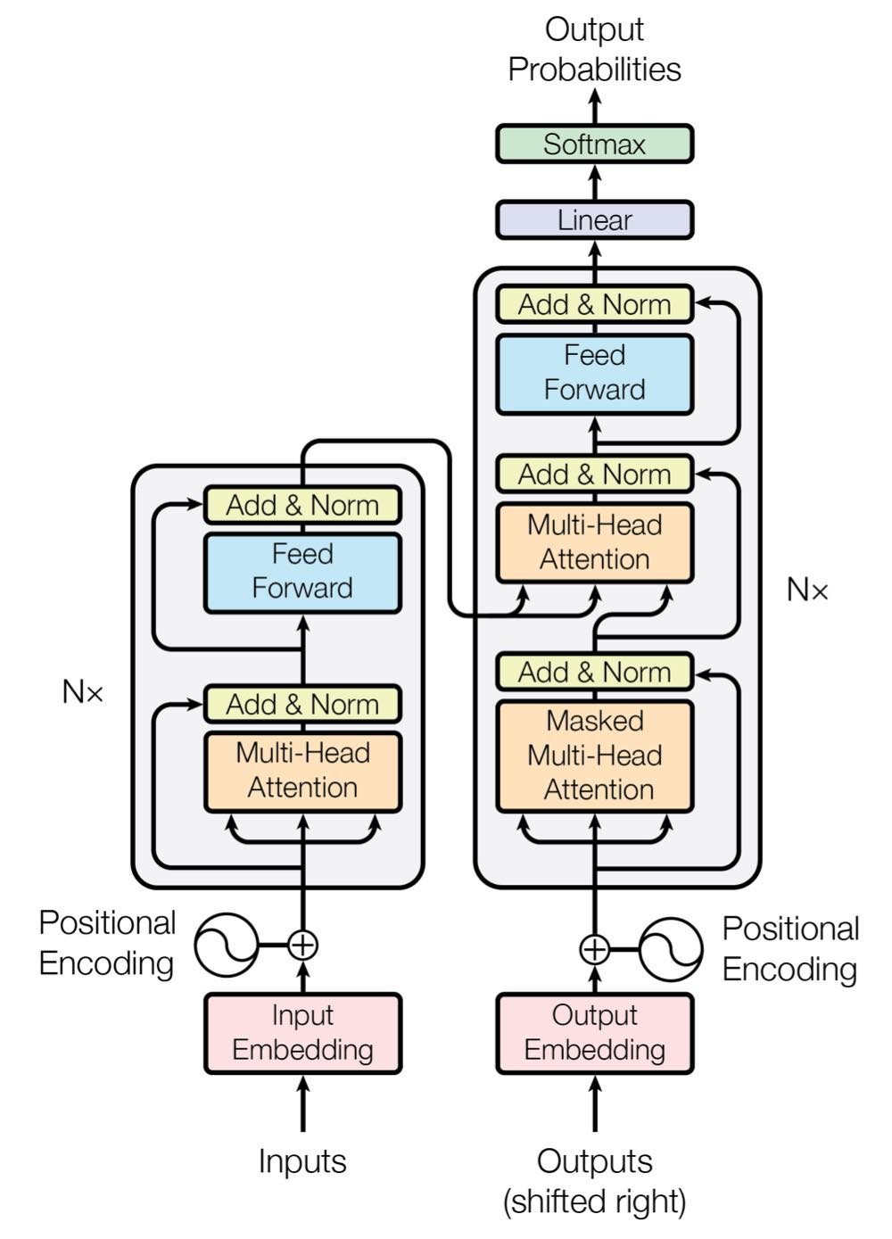
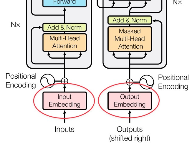
전반적으로 stacked self-attention과 point-wise를 사용하여 encoder-decoder 구조를 가지며, encoder, decoder 둘 다 위 사진과 같은 fully connected layers를 갖는다. (왼쪽 : encoder, 오른쪽 : decoder)
Encoder and Decoder Stacks
Encoder
먼저, encoder는 6개의 layer를 쌓은 형태로 이루어져 있고, 각 layer는 두 개의 sub-layer를 갖는다.
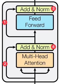
두 sub-layer는 각각 다음과 같다.
- Multi-head self-attention mechanism
- Position-wise fully connected feed-forward network
그림에서 1번, 2번 화살표는 residual connection을 나타낸다.
이는 ResNet에서 제안된 아이디어로, 특정 layer를 건너 뛰어서 입력해줌으로써 기존 정보에서 바뀐 잔여(residual)부분만 학습하도록 하여 초기 모델 수렴 속도를 높이며, global optima를 찾을 확률을 높여준다.
두 sub-layer 각각에 적용되며 이후에 normalization이 진행된다.
3번, 4번 과정은 각 sub-layer의 output이 나오는 단계로, \(\text{LayerNorm}(x + \text{Sublayer}(x))\)의 과정을 말한다.
Residual connection이 가능하도록 하기 위해, 모델 내의 모든 sub-layer들과 embedding layer들의 output dimension은 \(d_{\text{model}} = 512\)로 정한다.
Decoder
다음으로, decoder를 살펴보자.
Decoder 또한 6개의 layer로 이루어져 있다.
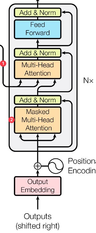
각 layer에는 2개의 sub-layer에 더하여 encoder의 output에 대해 multi-head attention을 수행하는 3번째 sub-layer가 존재한다. (1번 화살표와 연결된 multi-head attention)
그리고 subsequent position을 처리하지 않도록 multi-head attention 하나를 조금 수정하였는데, 이 layer를 Masked multi-head attention이라 한다. (2번)
Masking은 output embedding이 position 하나와 상쇄되어 position \(i\)에 대한 예측을 진행할 때 \(i\) 이전 position들에서의 known output에 대해서만 영향을 받도록 한다.
Attention
Attention 함수는 query 하나와 key-value 쌍들의 집합을 output으로 맵핑하는 과정으로 생각해볼 수 있다. (여기서 query, keys, values, output은 모두 벡터이다.)
특히 Transformer에서는 self-attention을 사용한다. 즉, input sequence(sentence)의 각 요소(token, 단어)들이 다른 어떤 요소와 연관성이 높은지를 학습하도록 만드는 것이다. 이를 통해 문맥에 대한 정보를 잘 학습하도록 한다.
Output은 value의 weighted sum으로 계산하며, 이때 weight은 query의 compatibility function과 각 value에 해당하는 key로 구한다.
이 과정을 좀 더 자세히 알아보자.
Scaled Dot-Product Attention
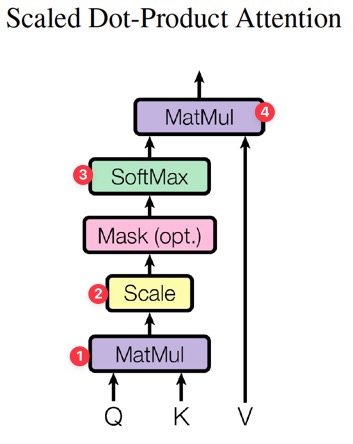
Scaled Dot-Product Attention은 Transformer에서 사용하는 특별한 형태의 attention이다.
차원 \(d_k\)인 query와 key를 input으로 받고, value의 차원은 \(d_v\)이다.
실제 attention function을 계산할 때, query의 set을 나타내는 matrix \(Q\), key와 value를 나타내는 \(K\)와 \(V\)를 사용하여 계산한다. 과정을 수식으로 나타내면 다음과 같다.
\( \text{Attention}(Q, K, V) = \operatorname{softmax}(\cfrac{QK^T}{\sqrt{d_k}})V \)
그림에서의 순서와 수식을 비교해보면 과정을 잘 이해할 수 있을 것이다.
그림에서 Query와 Key의 곱 및 softmax 과정이 이전 글에서 소개한 attention mechanism과 같다고 생각하면 된다.
(Attention에서는 이전 state \(s_{t-1}\)과 annotation \(h_j\)으로 구한 값인 energy의 비율을 softmax로 구하였다.)
대표적인 attention function 두 가지는 additive attention과 dot-product(multiplicative) attention이 있는데, Transformer에서는 후자에 scaling factor \(\cfrac{1}{\sqrt{d_k}}\)를 적용하여 사용한다. 이는 dot-product attention이 (최적화된 matmul code 덕에)훨씬 빠르고 공간을 효율적으로 사용하기 때문이다.
Scaling factor를 적용한 이유는, \(d_k\)가 커지게 되면 dot product의 규모가 커지게 되면서 softmax function의 graident가 매우 작아지는 현상이 발생하기 때문이다.
Multi-head attention
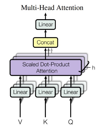
\(d_{\text{model}}\)차원의 key, value, query에 대해 attention function 하나만 수행하는 대신, 각각을 \(d_k, d_v, d_k\) 차원으로 \(h\)번 linearly project시키는 것이 효율적임을 발견했다. (이 projection도 parameter를 통해 학습된다.) 이 과정에서 query, key, value의 projected version 각각에 attention function을 parallel하게 적용하여 \(d_v\)차원의 output value를 얻는 것이다.
이렇게 얻은 결과를 연결하고 한 번 더 project하여 최종 결과값을 얻는다.
이러한 방법을 Multi-Head Attention이라 한다.
이 방법은 모델이 서로 다른 position에서의 representation subspace에 포함된 정보를 연결하여 처리할 수 있게 한다. (Single attention head에서는 평균을 구하므로 이러한 정보를 잃는다.)
Multi-Head Attention을 수식으로 표현하면 다음과 같다.
\( \text{MultiHead}(Q, K, V) = \operatorname{Concat}(\text{head}_1, \dots, \text{head}_h ) W^O \)
\( \text{head}_i = \operatorname{Attention}(QW_i^Q, KW_i^K, VW_i^V) \)
Projection의 parameter matrix의 차원은 각각
\(W_i^Q \in \mathbb{R}^{d_\text{model} \times d_k}, \; W_i^K \in \mathbb{R}^{d_\text{model} \times d_k}, \; W_i^V \in \mathbb{R}^{d_\text{model} \times d_v}, \; W_i^O \in \mathbb{R}^{h d_v \times d_\text{model}} \)이다.
논문에서는 head 개수를 \(h=8\)로 두었고, \(d_k=d_v=d_\text{model} / h = 64\)로 두었다.
각 head의 차원이 줄어들기 때문에 computational cost는 full 차원의 single-head attention의 computational cost와 비슷하다.
Three types of attention layer in Transformer
Transformer는 multi-head attention을 다음과 같은 세 가지 방법으로 사용한다. Transformer 전체 구조를 참고하며 알아보자.
- Encoder-decoder attention layer
- Query는 이전 decoder layer에서, key-value 쌍들은 encoder의 output에서 얻는다. 이를 통해 decoder의 모든 position이 input sequence의 모든 position을 처리할 수 있게 된다.
- 기존 seq2seq model의 전형적인 encoder-decoder attention mechanism과 같다.
- Encoder의 self-attention layer
- 모든 key, value, query는 이전 layer의 encoder output에서 얻는다. encoder의 각 position이 이전 encoder의 모든 position을 처리할 수 있게 된다.
- Decoder의 masked self-attention layer
- Decoder에서도 비슷하지만, decoder의 각 position이 현재 position까지 포함하여 그 이전까지의 모든 position을 처리할 수 있게 된다.
- Decoder에서는 auto-regressive property를 보존하기 위해 왼쪽으로 정보가 흘러들어가는 현상을 막아야 한다. 예를 들어, 앞 단어가 뒷 단어를 참고할 수 있도록 만들 경우 이것이 cheating과 같은 효과가 되어 모델이 정상적으로 학습되지 않는다.
- 이를 위해 scaled dot-product attention 과정에서 softmax 적용 이전에 input의 모든 value들을 masking(\(- \infty\)로 setting)하여 illegal connection의 효과를 부여한다.
Position-wise Feed-Forward Networks
다시 전체 아키텍쳐를 살펴보자.
앞서 두 가지 sub-layer가 있다고 하였다. Attention에 대해서 위에서 알아보았으니, 또다른 sub-layer인 Feed-Forward Network를 알아보자.
위 그림에서와 같이 encoder와 decoder 모두 fully connected feed-forward network를 갖고 있다. 이 신경망은 아래 수식과 같이 두 linear transformation의 RELU activation으로 이루어져 있다.
\( \text{FFN}(x) = \text{max}(0, x W_1 + b_1) W_2 + b_2 \)
서로 다른 position들에 대해서는 같은 linear transformation이 적용되지만, 각 layer에는 서로 다른 parameter를 사용한다. (마치 kernel size가 1인 두 convolution을 사용하는 것과 같다.)
input과 output의 차원은 \(d_\text{model} = 512\)이고, layer 내부에서는 차원 \(d_{ff} = 2048\)을 갖는다.
Embedding and Softmax
Input token과 output token을 \(d_\text{model}\) 차원의 벡터로 변환하기 위해 학습된 embedding을 사용한다.
이는 다른 sequence transduction model들과 비슷한 방식이다.
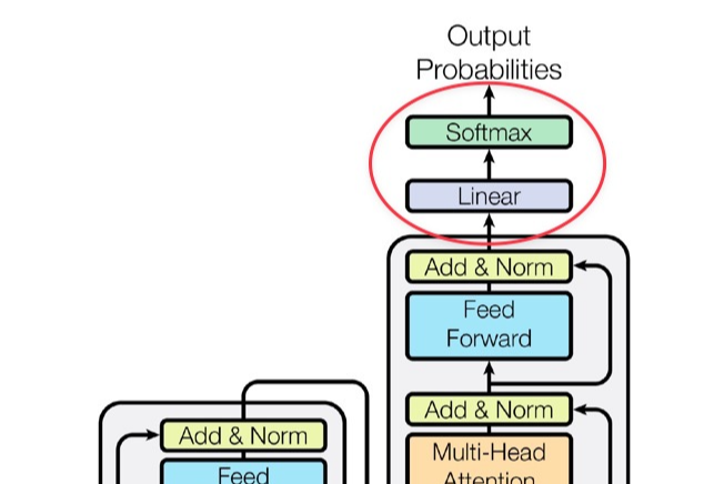
또한 decoder output을 통해 다음 token의 확률을 예측하기 위해 linear transformation과 softmax function을 사용한다.
특히 Transformer에서는 두 embedding layer와 softmax 이전의 linear transformation에 같은 weight matrix를 사용한다. (Embedding layer에서는 weights \(\sqrt{d_{\text{model}}}\)를 곱한다.)
사전 연구에서 output embedding을 통해 language model을 개선시킨 연구가 있다.
Positional Encoding
Transformer에는 recurrence와 convolution이 없기 때문에, model이 sequence의 순서를 다루도록 하기 위해서는 sequence 내에서 token의 위치에 대한 정보를 따로 주어야 한다. 이를 위해 사용하는 방법이 바로 positional encoding이다.
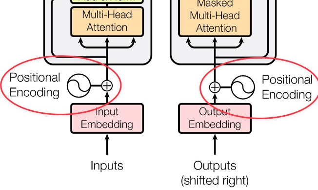
Positional encoding은 위 그림과 같이 encoder와 decoder stack의 아랫부분 (input embedding 부분)에 추가된다.
차원이 \(d_\text{model}\)로 embedding과 같은 차원을 가지므로, 서로 합(element-wise)할 수 있다.
여러 종류가 있는데, 논문에서는 아래와 같이 서로 다른 주파수를 갖는 sine과 cosine function을 사용했다.
\( \text{PE}_{(pos, 2i)} = \sin{( pos/10000^{2i/d_\text{model}} )} \)
\( \text{PE}_{(pos, 2i+1)} = \cos{( pos/10000^{2i/d_\text{model}} )}\)
여기서 \(pos\)는 position(단어의 위치)을, \(i\)는 차원(embedding의 위치)을 나타낸다.
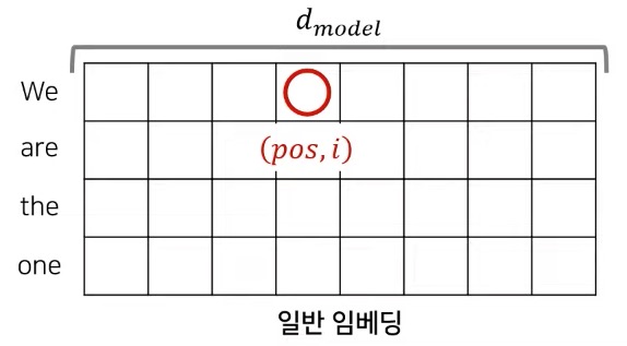
Positional encoding에서의 각 차원은 sin곡선에 해당하는 것이다. 파장은 \(2\pi\)에서 \(10000 \dot 2\pi\)까지 곡선을 그린다.
위 사진과 같은 embedding과 positional encoding을 element-wise로 더하여 encoder와 decoder의 입력으로 보내주게 된다.
sin, cos함수를 사용한 이유는 이 함수들을 사용하면 모델이 상대적 position을 다루도록 학습하기 쉬울 것이라는 가설을 세웠기 때문이다.
(고정된 offset \(k\)에 대해 \(\text{PE}_{pos + k}\)가 \(\text{PE}_{pos}\)의 linear function으로 표현 가능하기 때문이다.)
여러 경우에 대해 실험을 진행해 보았을 때, sinusoidal positional encoding을 사용했을 때와 learned positional embedding을 사용했을 때가 가장 이상적인 결과에 가까웠음을 알 수 있었다.
논문에서는 sinusoidal positional encoding을 사용했는데, 이를 통해 모델이 학습 도중에 처리하는 sequence보다 더 긴 길이의 sequence를 추론할 수 있기 때문이다.


최근댓글