Pointcloud-related Models (2) - PointNet++

 

목차

 

[논문 링크, Github 링크]

이전 포스팅에서 Point cloud 데이터를 직접적으로 다루는 최초의 모델인 PointNet 논문을 리뷰해보았다.

이번에는 이를 보완한 PointNet++ 모델을 제안한 논문 'Charles Ruizhongtai et al., PointNet++: Deep Hierarchical Feature Learing on Point Sets in a Metric Space'를 리뷰해보려 한다. Point를 직접적으로 다루는 모델의 원리를 공부해보기 위해 선택한 논문이므로 experiment에 대한 상세한 설명은 뺐다.

 

 

 

 

Motivation

 

PointNet은 point cloud data를 직접적으로 입력받아 point 각각의 feature와 global feature를 구한다. 이를 합하여 segmentation task를 수행하는데, local structure를 잘 잡아내지는 못한다. 즉, point 일부가 생성하는 미세한 패턴을 파악하거나 일반화하는 성능에서는 한계를 보인다.

CNN의 경우에는 locality principle이 존재하여, 작은 부분(local)부터 점차 큰 scale의 feature를 포착한다. 즉, 초기에는 neuron의 receptive field가 작고, layer를 거칠수록 receptive field가 커진다.

이러한 개념을 PointNet에 적용한 모델이 바로 PointNet++ 모델이다.

 

 

 

 

Introduction

 

 

 

Overview

 

Fig 1. PointNet++ Architecture

 

PointNet++의 가장 큰 특징은 계층적으로 feature를 잡아낸다는 것이다. (Hierarchical feature learning)

어떻게 hiearchical feature learning을 구현했는지 알아보자.

1. Input point set을 조금씩 겹치도록 나누어 각각에 PointNet을 적용한다.
2. Point 간의 distance를 고려하며, scale을 증가시키면서 local feature를 학습한다.

이를 통해 부분적인(local) feature를 잘 잡아내고, layer를 거칠수록 feature의 범위가 커지게 된다. 또한 여러 scale의 feature를 학습하므로 robustness도 증가한다.

 

 

 

Two Issues of Designing PointNet++

 

이러한 PointNet++를 설계하기 위해서는 두 가지를 고려해야 한다.

1. Point set을 어떻게 나눌 것인가?
2. Point set 혹은 local feature를 어떻게 학습할 것인가?

 

Local feature learner  → PointNet

먼저, 각 layer에서 feature를 학습하는 모델로는 PointNet을 활용한다.

 

Fig 2. Use PointNet as a Local Feature Learner

 

CNN에서 window 크기에 따라 이미지를 부분으로 나눈 후, 해당 window에서 local feature를 계산하듯이, PointNet++에서는 point set을 특정 기준으로 나눈 후, 그 subset들에 PointNet을 통해 local feature를 계산한다. 이때, CNN에서처럼 local feature learner(PointNet)의 weight는 공유가 가능하다.

 

Overlapping partitioning

그리고 처음 layer에서 PointNet을 적용하기 전에 point set을 일정 기준을 갖고 subset으로 나눠주어야 할 것인데, 이때 사용하는 방법이 바로 opverlapping partitioning이다.

 

Fig 3. Partitions before Applying PointNet

 

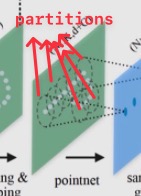
여기서 partition이란, Euclidean space(3차원 공간)에서의 구를 말하며, centroid 위치(location)와 크기(scale) 등으로 정의한다. Overlapping partitioning에서는 두 parameter를 다음과 같이 정한다.

• Location of centroid : Farthest Point Sampling (FPS) 알고리즘을 적용한다.
• Scale : Point set의 특성 상, 영역마다 density가 다르다는 점을 고려하여 적절한 scale로, 조금씩 겹치도록 partition을 정해야 한다.
  • CNN에서는 kernel size가 작을수록(미세한 local feature를 잡아낼수록) 성능이 높아지지만, PointNet++에서는 구의 지름이너무 작아질 경우 속한 point의 개수가 너무 적어 성능이 떨어진다.

 

Volumetric CNN과 PointNet++를 비교해봤을 때, volumetric CNN은 고정된 voxel grid를 사용하지만, PointNet++에서는 input data의 특성과 metric을 둘 다 고려한, 유연한 receptive field를 사용하기 때문에 더 효율적이고, 효과적이다.

 

 

 

 

Method

 

PointNet++가 어떤 방법으로 동작하는지 자세히 알아보자.

 

Fig 1. PointNet++ Architecture

 

설명을 위해 사용할 용어는 다음과 같다.

• \(\mathcal{X} = (M, d) \) : Euclidean space \(\mathbb{R}^n\)의 discrete metric space → 쉽게 생각해서 3D object point cloud 혹은 3D scene point cloud
  • \(M \subset \mathbb{R}^n\) : Point set (density가 일정하지 않음)
  • \(d\) : Distance
• \(f\) : Objective function → PointNet의 universal continuous set function
  • Input : \(\mathcal{X}\) 및 point 별 추가적인 feature(x, y, z 좌표 이외의 feature)
  • Output : \(\mathcal{X}\)와 관련된 semantic 정보
    • Classification → \(\mathcal{X}\)의 label
    • Segmentation → Point 각각의 semantic label

 

 

 

PointNet (Review)

 

PointNet을 간단하게 복습해보자. PointNet은 주어진 point cloud(unordered set \(\{x_1, x_2, \dots, x_n \}, \; \text{where } x_i \in \mathbb{R}^d \))에 대해 다음 set function(point를 vector로 맵핑하는 함수 \(f : \mathcal{X} \rightarrow \mathbb{R}\))을 근사하는 모델이다.

\( f(x_1, x_2, \dots, x_n) = \gamma \left( \underset{i=1, \dots, n}{\max} \{h(x_i)\} \right) \)

• \(\gamma, h\) : 서로 다른 MLP network, 특히 \(h\)의 결과는 각 point의 spatial encoding

 

이러한 set function(max pooling function)은 input point의 순서에 invariant하고, 어떠한 continuous set function도 근사가 가능하다는 특징을 갖는다.

하지만 앞에서도 언급했듯이, 다양한 scale에서의 local context를 잡아내는 능력은 부족하다. 따라서 hierarchical feature learning 방법으로 이 한계를 해결해보고자 한다.

 

 

 

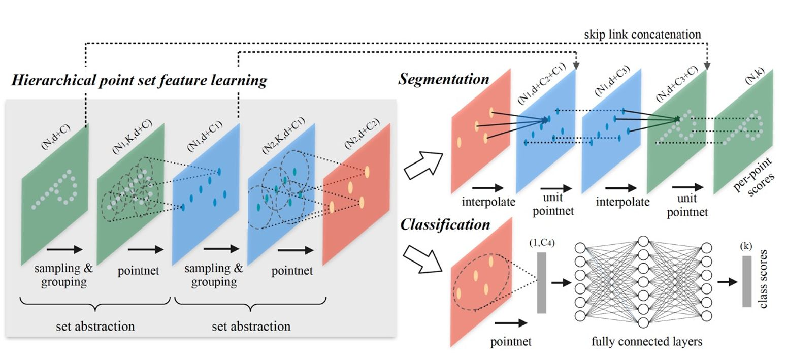
Hierarchical Feature Learning (Set Abstraction)

 

PointNet에서는 전체 point set에 대해 max pooling 연산 한 번만 진행했으나, PointNet++에서는 point set을 (계층을 지날 때마다 점점 커지는) partition으로 나누어 점점 넓은 지역에서의 local feature를 학습한다.

 

Fig 4. Hierarchical Point Set Feature Learning

 

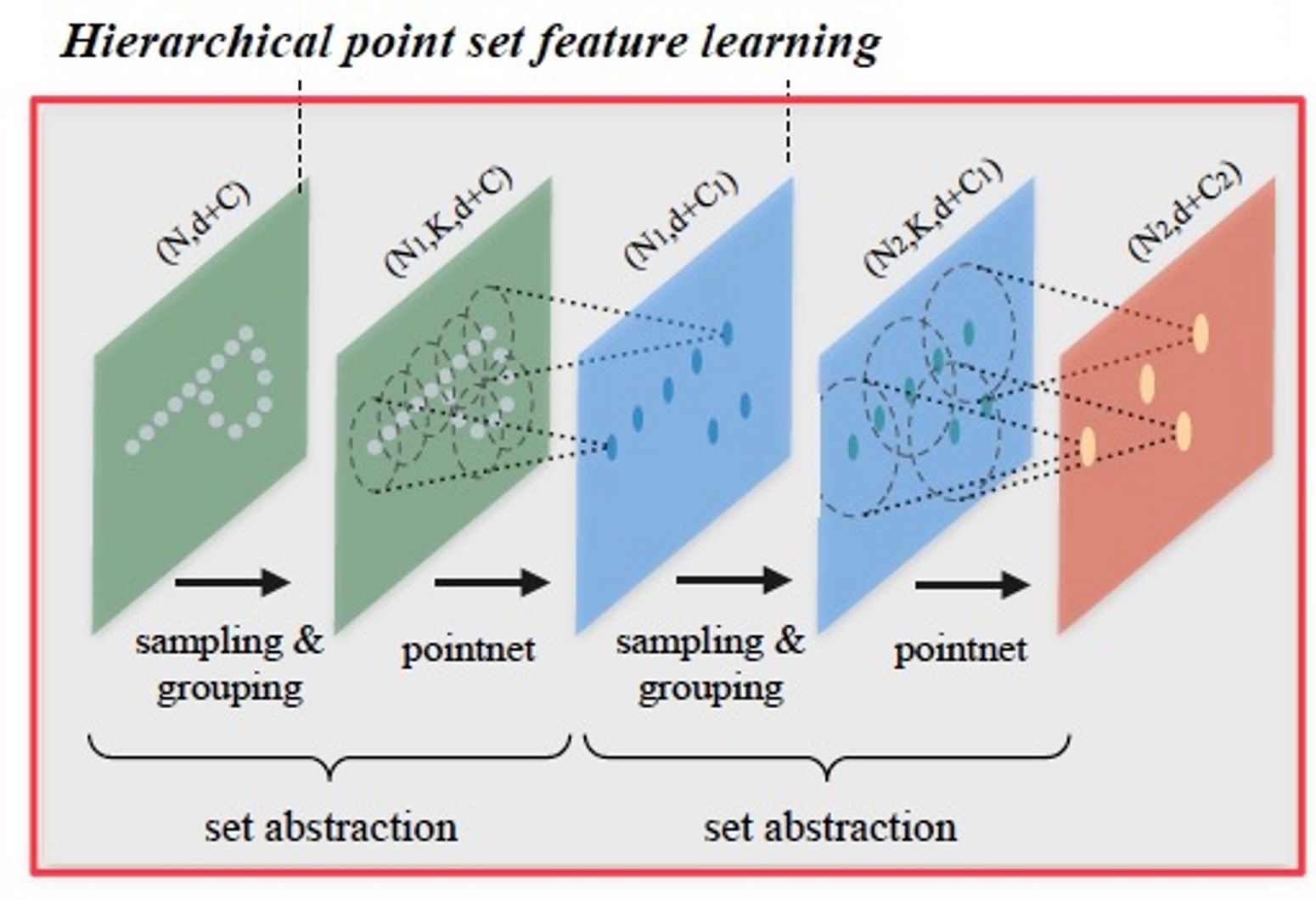
Fig 4는 이러한 hierarchical feature learning 과정을 보여준다. Set abstraction 부분이 각 계층(hierarchy)에서 scale에 따른 local feature를 얻는 과정이다. 당연히 계층을 지날수록 element 수는 줄어들 것(\(N > N_1 > N_2\))이고, scale(partition의 범위)은 커질 것이다.

Set abstraction level(첫 번째)안에서 point를 처리하는 과정(sampling layer → grouping layer → PointNet layer)을 자세히 알아보자.

• Shape of input matrix : \(N \times (d + C)\)
  • \(N\) : Point 개수
  • \(d\) : Coordinates 차원
  • \(C\) : Point feature의 차원
• Shape of output matrix : \(N^\prime \times (d + C^\prime)\)
  • \(N^\prime\) : Subsampling된 point set의 개수
  • \(d\) : Coordinates 차원
  • \(C^\prime\) : 새로운 point feature의 차원

 

1. Sampling layer

Sampling layer는 input point들로부터 point set을 골라내는 과정, 즉 partition의 centroid를 정의하는 과정이다.

이때 Farthest Point Sampling(FPS) 알고리즘을 사용하여 주어진 input points \(\{x_1, x_2, \dots, x_n\}\)에 대해 subset \(\{x_{i_1}, x_{i_2}, \dots, x_{i_m}\}\)을 고른다. 여기서 \(x_{i_j}\)는 set \(\{x_{i_1}, x_{i_2}, \dots, x_{i_{j-1}}\}\)을 제외하고 남은 점 중에서 모든 set과의 거리가 가장 먼 점을 말한다.

 

Fig 5. 'i'th iteration of FPS

 

CNN을 적용할 때에는 data 분포에 상관 없이 공간을 나누지만, FPS를 사용할 경우 data 분포에 따라 receptive field를 생성하게 된다.

 

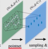
2. Grouping layer

Grouping layer는 centroid 주변의 점들을 묶어 partition(local region set)을 구성하는 단계이다. 이를 거치면서 input shape \(N \times (d + C)\)이 \(N^\prime \times K \times (d + C)\)로 바뀌게 된다.

이때 \(K\)는 각 centroid point와 grouping된 주변(이웃) 점의 개수이다. parition에 따라 \(K\)가 다른데, PointNet layer에 의해 같은 차원의 feature vector로 맵핑된다.

 

Fig 6. Grouping process

 

Grouping을 하기 위한 알고리즘에는 kNN(k Nearest Neighbor) searching algorithm(고정된 이웃 점 개수 찾음)이나 ball query(query point에 대해 반지름 이내의 point들을 찾음) 등이 있는데, PointNet++에서는 region scale이 고정되고, 그 고정된 공간에 대한 feature를 뽑을 수 있는 ball query 방법을 주로 사용한다.

CNN은 Manhattan distance(kernel size)로 정해진 크기의 local region을 가지는데 반해, PointNet++에서의 partition은 point set이 metric space(3차원 공간)에 존재하므로 이웃 점은 metric distance로 정의된다.

 

3. PointNet layer

이제 PointNet을 사용하여 각 local region의 feature를 뽑는다. Input shape은 \(N^\prime \times K \times (d + C)\), output (feature) shape은 \(N^\prime \times (d + C^\prime)\)이다.

과정은 다음과 같다.

1. Relative coordinate : Local region(partition)에 포함된 점들의 coordinate를 centroid 기준의 local frame으로 변환한다.
   • \(\mathbf{x}_i^{(j)} = \mathbf{x}_i^{(j)} - \hat{\mathbf{x}}^{(j)}, \; \text{for } i=1, 2, \dots, K \; \text{and } j = 1, 2, \dots, d\)
     • \(\hat{\mathbf{x}}\) : Centroid의 coordinate
     • \(K\) : Partition(local region)에 포함된 point 개수 (centroid 제외)
   • 이 과정을 통해 local region 내에서의 point 간의 관계를 포착할 수 있다.
2. PointNet을 적용하여 local region의 feature를 얻는다.

 

 

 

Robust Feature Learning

 

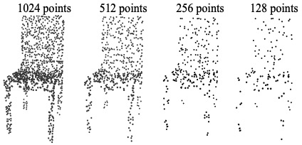
앞서 언급했듯, point set의 특징은 같은 부피의 공간에 일정한 밀도로 point가 존재하지 않는다는 것이다. (Non-uniform sampling density)

따라서 feature learning이 어렵다. 예를 들면, 점이 dense한 곳에서 얻은 feature는 sparse한 곳에 사용할 수 없을 것이다. 즉 sparse point cloud에 대해 학습한 모델은 미세한 local structure를 인지할 수 없을 것이다.

이를 해결하기 위해 PointNet++에서는 (density) adaptive PointNet layer를 사용한다. 이는 point density에 따라 다양한 abstraction level을 사용하여 여러 scale의 feature를 뽑고, 이를 결합하는 방법이다.

즉, 위에서 설명했던 abstraction level에서는 단일 scale에 대한 grouping과 feature extaction을 진행했는데, 실제로 PointNet++에서는 non-uniform sampling density 문제를 해결하기 위해 abstraction level 각각에서 여러 scale에 대한 feature를 뽑고 local point density를 고려하여 그것을 결합한다.

 

Fig 7. Multi-Scale Grouping (MSG, a) and Multi-Resolution Grouping (MRG, b)

 

Fig 7과 같이 Adaptive PointNet layer에는 grouping과 combining 방식에 따라 MSG, MRG 두 가지 종류가 있다.

 

MSG(Multi-Scale Grouping)

Multi-Scale Grouping(MSG)이란, 다양한 scale의 local region에 대해 grouping layer를 적용한 후에 PointNet layer로 각각의 scale에 대한 feature를 뽑은 후 concat하는 방법이다.

 

Fig 8. Random point dropout

 

Training 시에는 instance마다 input point를 랜덤하게 dropout하는 random input dropout 기법을 사용한다. 이는 training point set마다 다른 비율로 dropout을 적용하여 다양한 density의 training set에 대해 학습을 진행하는 효과를 얻기 위해서이다. (기존 dropout과 마찬가지로 test 시에는 dropout을 적용하지 않는다.)

하지만, 이 방법의 경우 모든 partition의 centroid에 대해 PointNet을 적용해야 하므로 computational cost가 높다는 단점이 있다. 특히 초반 단계에서는 centroid(partition)가 매우 많으므로 계산량이 아주 높다.

 

MRG(Multi-Resolution Grouping)

Multi-Resolution Grouping(MRG)이란, 어떤 level(layer) \(L_i\)에서의 region(partition)에 대한 feature를 아래 두 vector를 concat하여 얻는 방법을 말한다.

1. 이전 level \(L_{i-1}\)의 각 subregion(partition)에 대한 feature의 summarization vector
2. 모든 raw point에 PointNet을 적용하여 얻은 feature

Concat 시에 weight을 부여하는데, local region이 sparse한 경우에는 subregion은 더 sparse하기 때문에 2번 벡터에 높은 weight을 부여하고, local region이 dense한 경우에는 이전 level에서 더 detail한 정보를 제공하므로(더 높은 resolution을 처리하므로) 1번 벡터에 높은 weight을 부여한다.

이 방법은 첫 단계에서 large scale의 feature를 뽑지 않기 때문에 계산량 측면에서 효율적이다.

 

 

 

Point Feature Propagation for Segmentation

 

Fig 9. Feature Propagation for Segmentation

 

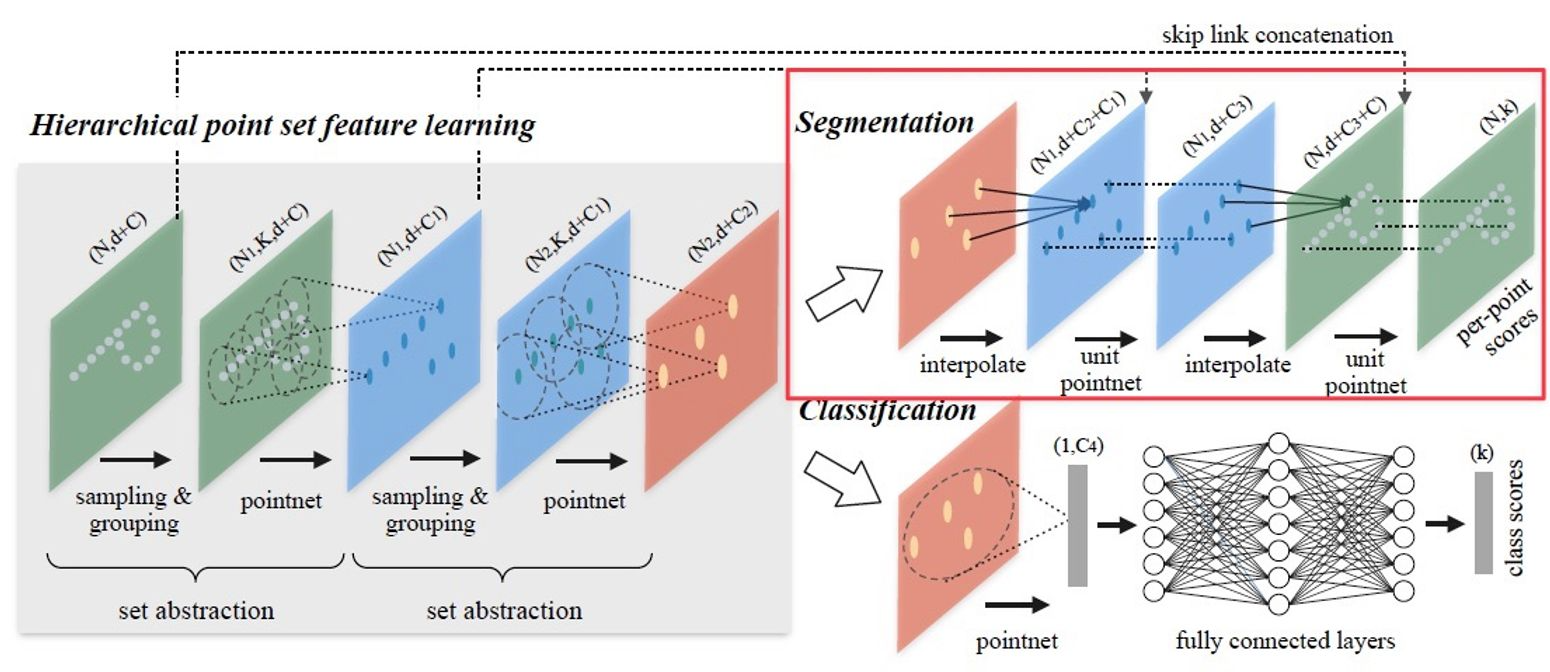
PointNet에서와 마찬가지로, segmentation task를 수행하기 위해서는 모든 point 각각에 대한 segment label score가 필요하다. 따라서 subsampling했던 point feature를 원래의 point로 전파(propagate)하는 과정이 필요하다.

Feature propagation 과정의 핵심은 interpolation과 skip link concatenation이며, original point set의 feature를 얻을 때까지 반복적으로 이루어진다. Hierarchical propagation 과정과 반대로, input point feature shape은 \(N_l \times (d + C)\), output point feature 개수는 \(N_{l-1} (\text{where } N_l \leq N_{l-1})\)이라 하자.

(Fig 9에서 보듯, feature learning(hiearchical propagation) 시 set abstraction 횟수와 feature propagation 반복 횟수가 같을 것이다.)

 

Interpolation

Interpolation이란, \(L_l\) level에서 \(N_l\)개 point의 feature value들에 interpolation을 적용하여 \(L_{l-1}\) level의 \(N_{l-1}\)개 point의 feature value를 계산하는 방법이다. 여러 interpolation 방법 중 K Nearest Neighbors 기반의 inverse distance weighted average를 사용한다.

\( f^{(j)}(x) = \cfrac{\sum_{i=1}^k w_i(x) f_i^{(j)}}{\sum_{i=1}^k w_i(x)} \quad \text{where } w_i(x) = \cfrac{1}{d(x, x_i)^p}, \; j = 1, \dots, C \)

Default로 \(p = 2, k = 3\)을 적용했다. 즉, 2차 inverse distance를 사용하였고, \(L_l\) level에서 point 3개에 대해 interpolation을 적용한 것이다.

 

 

 

 

Experiments

 

중요한 결과 위주로 간단히 살펴보자.

 

 

Shape Classification

 

Fig 10은 ModelNet40(3D object classification task에서 사용하는 dataset)에 대한 성능 비교 결과이다.

 

Fig 10. ModelNet40 Shape Classification Results

 

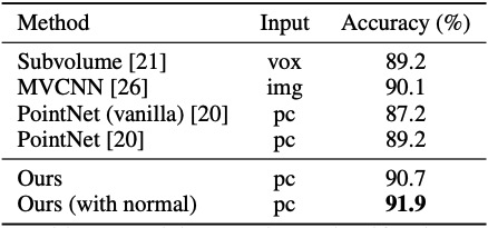
PointNet(vanilla)는 Transformation network를 사용하지 않은, 즉 PointNet++의 hieararchical network에서 abstraction level 한 번만 적용한 것과 같다.

PointNet과 비교했을 때, hierarchical architecture를 적용한 결과 3D object classification 성능이 더 좋아졌음을, CNN 기반 방법인 MVCNN보다 point set 기반 방법이 성능이 더 좋음을 알 수 있다. (마지막 행에서 normal information이란, input point feature로 face normal을 추가한 것이다.)

 

Fig 11. Advantage of Density Adaptive Strategy

 

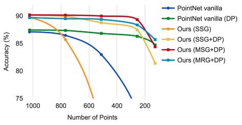
Fig 11은 sampling density variation(non-uniform density)에도 강인한지를 알려주는 실험 결과이다.

Density adaptive PointNet layer를 사용한 방법(MSG+DP → Multi-Scale Grouping + random input Dropout, MRG+DP → Multi-Resolution Grouping + random input Dropout)이 아주 robust함을 알 수 있다. SSG는 Single Scale Grouping의 줄임말로, adaptive PointNet layer를 사용하지 않은 버전이다.

 

 

 

Semantic (Scene) Segmentation

 

Scene에 대한 labeling을 진행한 결과도 살펴보자.

 

Fig 12. ScanNet Labeling Accuracy

 

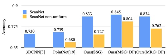
3DCNN은 voxel 기반의 CNN을 활용하는 모델이다. 꽤 큰 성능 변화가 일어났음을 알 수 있다. Voxel 기반 방법과 비교했을 때에는 (point cloud에서 직접적으로 학습하기 때문에)quantization error의 영향을 덜 받고, data distribution에 따라 sampling을 진행하므로 성능이 좋아졌을 것이고, PointNet과 비교했을 때에는 hierarchical architecture를 통해 다양한 크기의 object를 더 잘 이해함으로써 성능이 좋아졌다.

또한, adaptive PointNet layer를 통해 non-uniform density 특성에도 강인한(Fig 12의 파란 색과 노란 색의 차이가 확 줄어든) 모습을 보였다.

 

Fig 13. ScanNet Labeling Results

 

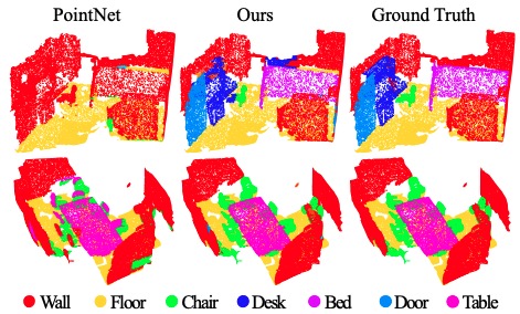
Fig 13을 통해 PointNet도 방의 전체적인 모습은 잘 포착을 하지만, detail한 가구들은 PointNet++에 비해 잘 포착해내지 못함을 알 수 있다.

 

 

 

Point Set Classification in Non-Euclidean Metric Space

 

PointNet++는 Euclidean space가 아닌 point set에 대해서도 잘 동작한다.

 

Fig 14. Example of Non-rigid Shape Classification

 

Non-rigid shape classification을 잘 수행하는 모델은 왼쪽(말)과 오른쪽(말)이 pose는 달라도 같은 category이고, 왼쪽(말)과 가운데(고양이)가 비슷한 pose를 취하고 있으나 다른 category임을 구분할 수 있어야 한다. 이는 intrinsic structure를 잘 학습하는지를 알아보는 task이다.

 

Fig 15. SHREC15 Non-rigid Shape Classification

 

Fig 15는 SHREC15 dataset을 통해 이러한 non-rigid shape classification 성능을 비교한 결과이다.

1번의 경우 이제까지 알아본 PointNet++에서처럼 Euclidean metric space를 기반으로(XYZ coordinate만 input으로 사용하여) point feature를 얻은 것이고, 이는 pose의 영향을 많이 받기 때문에 성능이 현저히 떨어짐을 알 수 있다.

반면 2번은 Euclidean metric space를 기반으로 intrinsic feature를 얻은 방법, 3번은 Geodesic distance를 기반으로 intrinsic feature를 얻은 방법이다. (자세한 방법은 논문을 참고하자.)

DeepGM도 3번과 비슷하게 geodesic moment를 shape feature로 활용하는 SOTA 방법이다. 하지만 PointNet++가 더 좋은 성능을 보임을 알 수 있다.