딥러닝 기초 - RNN (2)

 

목차

 

자주 잊어버리는 딥러닝 기초 내용을 여러 포스팅에 걸쳐 간단하게 정리해보려 한다. 다룰 내용은 크게 아래와 같다.

• Introduction
• Elements of ML
• Multi-layer Perceptron
• Model Selection
• CNN
• GNN
• RNN

 

 

이번에는 이전 글에 이어 RNN의 단점을 보완한 LSTM과 GRU에 대해 알아볼 것이다.

먼저 RNN의 feed-forward 수식과 single unit 그림은 다음과 같다. (activation function은 tanh 대신 다른 것을 사용할 수 있다.)

\( \mathbf{h}_t = f_{w_h} (\mathbf{x}_t, \mathbf{h}_{t-1}) \)
\( \mathbf{o}_t = g_{w_o} (\mathbf{h}_t) \)

 

Fig 1. RNN

 

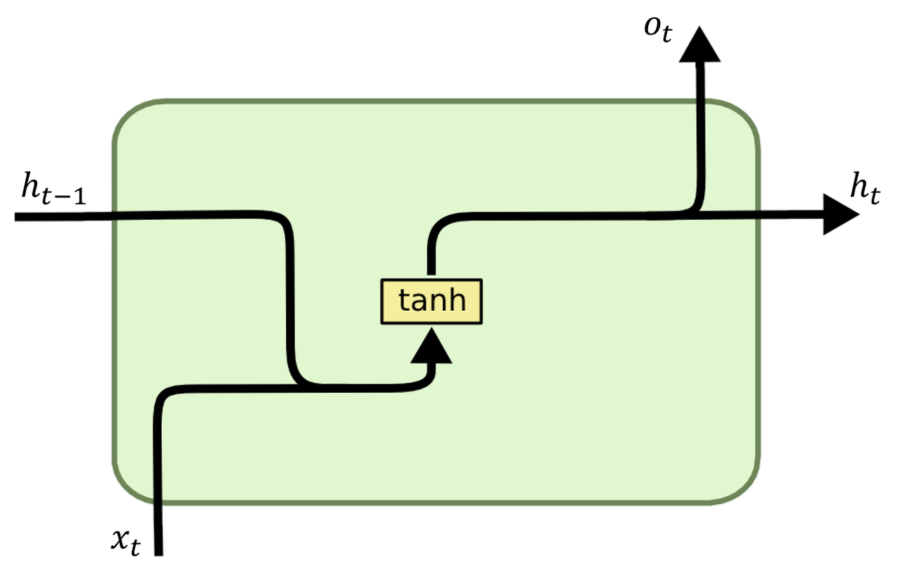
이전 글에서도 언급했듯, RNN의 문제점은 Long-term dependency가 떨어진다는 것이다. 예를 들어, 문장을 입력으로 받는다고 했을 때, 문장이 길어지면 마지막 단어가 첫 단어의 영향을 거의 받지 않게 된다.

이를 해결한것이 LSTM이고, LSTM을 간소화한 것이 GRU이다. 각각을 자세히 살펴보자.

 

 

 

Long-Short Term Memory (LSTM)

 

LSTM에서는 여러가지 gate와 memory cell이라는 개념을 사용하여 연산이 이루어진다. 특히, memory cell을 사용하여 초기의 input 정보까지도 저장하여 끝까지 영향을 줄 수 있도록 하였다.

LSTM의 feed-forward 과정의 수식과 single unit을 살펴보자.

\( \mathbf{H}_t = \mathbf{O}_t \odot \tanh (\mathbf{C}_t) \)
\( \mathbf{C}_t = \mathbf{F}_t \odot \mathbf{C}_{t-1} + \mathbf{I}_t \odot \tilde{\mathbf{C}}_t \)
\( \tilde{\mathbf{C}}_t = \tanh (\mathbf{X}_t \mathbf{W}_{xc} + \mathbf{H}_{t-1} \mathbf{W}_{hc} + \mathbf{b}_c) \)
\( \mathbf{I}_t = \sigma (\mathbf{X}_t \mathbf{W}_{xi} + \mathbf{H}_{t-1} \mathbf{W}_{hi} + \mathbf{b}_i) \)
\( \mathbf{F}_t = \sigma (\mathbf{X}_t \mathbf{W}_{xf} + \mathbf{H}_{t-1} \mathbf{W}_{hf} + \mathbf{b}_f) \)
\( \mathbf{O}_t = \sigma (\mathbf{X}_t \mathbf{W}_{xo} + \mathbf{H}_{t-1} \mathbf{W}_{ho} + \mathbf{b}_o) \)

• \( \mathbf{I}_t, \mathbf{F}_t, \mathbf{O}_t \) : Input gate, Forget gate, Output gate
• \( \mathbf{C}_t, \tilde{\mathbf{C}}_t \) : Memory cell, Candidate memory cell
• \( \mathbf{H}_t \) : Hidden state
• \( \odot\) : Hadamard product (elment-wise 곱)
• \( \sigma \) : Activation function을 갖는 fully connected layer

 

Fig 2. LSTM

 

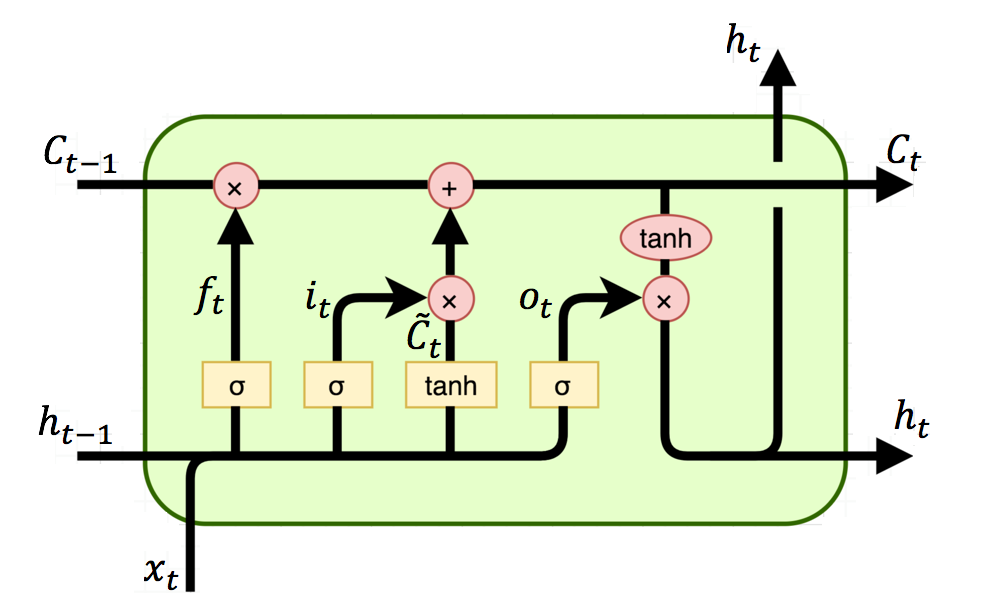
Memory cell state는 long-term dependency를 부여하는 핵심이며, 정보를 계속해서 흐르게 해준다. Input, forget gate에 영향을 받으며, output gate와 함께 hidden state를 결정한다.

Input gate는 data를 언제, 얼마나 읽을지를 결정하고, forget gate는 어떤 정보를 버릴지 정하며, output gate는 어떤 정보를 hidden state로 넘길지 정한다. (Sigmoid activation function을 통해 0~1 사이의 값을 내보낸다.)

 

 

 

 

 

 

Gated Recurrent Units (GRU)

 

GRU는 LSTM의 long-term dependency 성능을 유지하면서 복잡한 구조를 좀 더 단순화한 모델이다.

마찬가지로 수식과 그림을 통해 이해해보자.

\( \mathbf{H}_t = \mathbf{Z}_t \odot \mathbf{H}_{t-1} + (1 - \mathbf{Z}_t) \odot \tilde{\mathbf{H}}_t \)
\( \tilde{\mathbf{H}}_t = \tanh(\mathbf{X}_t \mathbf{W}_{xh} + (\mathbf{R}_t \odot \mathbf{H}_{t-1} ) \mathbf{W}_{hh} + \mathbf{b}_h ) \)
\( \mathbf{R}_t = \sigma(\mathbf{X}_t \mathbf{W}_{xr} + \mathbf{H}_{t-1} \mathbf{W}_{hr} + \mathbf{b}_r ) \)
\( \mathbf{Z}_t = \sigma (\mathbf{X}_t \mathbf{W}_{xz} + \mathbf{H}_{t-1} \mathbf{W}_{hz} + \mathbf{b}_z ) \)

• \( \mathbf{H}_t, \tilde{\mathbf{H}}_t \) : Hidden state, Candidate hidden state
• \( \mathbf{R}_t, \mathbf{Z}_t \) : Reset gate, update gate

 

Fig 3. GRU

 

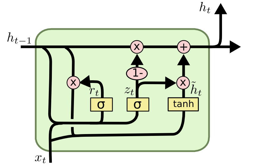
GRU에서는 cell state와 hidden state를 hidden state \(\mathbf{H}\)로 합쳤고, update gate \(\mathbf{Z}\)로 LSTM의 forget gate와 input gate 개념을 합쳐 hidden state(cell state)에 어떤 정보를 얼마나 반영해줄지를 고려한다.

 

 

LSTM과 GRU 이외에도 hidden state의 앞, 뒤로, 즉 정보를 양방향으로 전달할 수 있는 bidirectional RNN도 존재한다. 이는 최근 GPT와 함께 아주 좋은 성능을 내고 있는 BERT 모델의 기초 개념이다. (단, bidirectional RNN을 무턱대고 사용하다간 오히려 나쁜 성능을 보일 수 있으며, 학습 속도가 매우 느리므로 유의해서 사용해야 한다.)