Tensor의 shape을 가독성있게 변환하는 einops 사용법

 

 

목차

 

 

인공지능 연구를 하면서 코딩을 하다보면 Numpy, PyTorch, Tensorflow 등의 tensor의 shape을 변환해주는 경우가 매우 많다. 필자의 경우 PyTorch를 가장 많이 사용하는데, reshape(), view(), squeeze() 등등 tensor shape을 변환하는 함수의 종류도 너무 다양하고, 가독성도 떨어진다. 또한 변환된(또는 변환 할) tensor의 현재 shape이 어떤지 알 수 없기 때문에 디버깅할 때에도 매우 불편하다.

우연히 이를 깔끔하게 해결해줄 수 있는 einops라는 라이브러리를 알게되어 자주 쓰는 함수 위주로 내용을 간단히 정리해보려 한다.

우선, 공식 홈페이지에 가보면 document와 함께 추가적인 정보를 알 수 있다.

https://einops.rocks/

Einops

 

 

 

einops

 

 

 

Installation

 

# with anaconda
conda install -c conda-forge einops
# with pip
pip install einops

 

 

 

유용한 함수

 

einops는 문자열을 활용하여 tensor의 shape을 직관적이고 가독성 있게 변형해준다. pytorch나 numpy에서 제공하는 transpose, permutation, reshape, view, squeeze, unsqueeze, stack, concatenate 등의 함수를 대체할 수 있다.

 

 

 

rearrange()

 

from einops import rearrange
# ex) list of 32 images with (h, w, c) = (30, 40, 3)
input_tensor = [np.random.randn(30, 40, 3) for _ in range(32)]
# list to numpy array (stack along batch axis)
output_tensor = rearrange(input_tensor, "b h w c -> b h w c") # (32, 30, 40, 3)
# reshape (concat along height axis)
output_tensor = rearrange(input_tensor, "b h w c -> (b h) w c") # (960, 40, 3)
# reshape (reordering)
output_tensor = rearrange(input_tensor, "b h w c -> b c h w") # (32, 3, 30, 40)
# flatten (each image into a vector)
output_tensor = rearrange(input_tensor, "b h w c -> b (c h w)") # (32, 3600)
# split -> 괄호 내의 순서는 상관 없음
output_tensor = rearrange(input_tensor, "b (h1 h) (w1 w) c -> (b h1 w1) h w c", h1=2, w1=2) # to batch: (128, 15, 20, 3)
output_tensor = rearrange(input_tensor, "b (h h1) (w w1) c -> b h w (c h1 w1)", h1=2, w1=2) # to channel: (32, 15, 20, 12)

 

string으로 shape을 표시해줄 때 에러를 주의해야 한다. 특히 띄어쓰기는 필수적으로 지켜야 한다.

Error example

 

 

Contiguous() 붙여줘야 하는 경우

일반적으로, PyTorch의 텐서의 shape을 변경해줄 때, view 함수를 사용하는 경우에는 contiguous()를 붙여주지 않으면 에러가 뜬다.

rearrange 함수의 경우 view와 비슷하게 동작하도록 pattern을 설정해줄 수 있는데, 이 때 contiguous()를 붙여주지 않으면 (DDP를 돌릴 때) warning이 뜬다. (사실 학습을 돌리는 데 큰 지장이 없지만, 느려질 수 있다는 에러 문구가 상당히 거슬린다.)

contiguous()를 붙여주지 않아 발생한 경고 문구

 

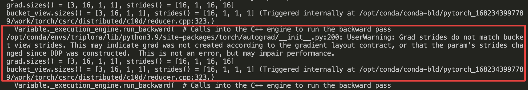
아래 예시를 보자.

a = rearrange(a, "(n b) h w c -> b h (w n) c", n=number).contiguous() # 필수!
b = rearrange(b, "b h (w n) c -> (n b) c h w", n=number).contiguous() # 필수!

c = rearrange(c, "n b h w c -> (n b) h w c") # 없어도 됨
d = rearrange(d, "(n b) h w c -> n b h w c") # 없어도 됨
e = rearrange(e, "(n b) p c h w -> n (b p) c h w", n=number) # 없어도 됨

 

정확한 이유는 contigous()가 필요한 이유(메모리가 어쩌고 저쩌고..)까지 공부를 해야하는 것 같아 넘어가고, 어림 짐작 하기로는 예시의 a, b를 보면, 첫 번째 dimension의 일부가 세 번째 dimension의 일부로 옮겨가거나, 그 반대인 경우이다. 이 경우가 view와 같은 역할을 하는 경우(contiguous가 필요한 경우)이다.

 

혹시 또 다른 경우가 발견되거나, 정확한 이유를 알게되면 내용을 추가하도록 하겠다.

 

 

 

reduce()

 

이 함수는 min, max, sum, mean, prod 등의 연산을 통해 특정 축을 없애거나 차원을 줄일 수 있다.

from einops import reduce
x = np.random.randn(10, 20, 30, 40)

# max reduction on the first axis
y = reduce(x, "b h w c -> h w c", "max") # (20, 30, 40)

# 2d max pooling with kernel size = 2 * 2 (image processing)
y1 = reduce(x, "b c (h1 h2) (w1 w2) -> b c h1 w1", "max", h2=2, w2=2) # (10, 20, 15, 20)

# adaptive 2d max pooling to 3 * 4 grid
y2 = reduce(x, "b c (h1 h2) (w1 w2) -> b c h1 w1", "max", h1=3, w1=4) # (10, 20, 3, 4)

# global avg pooling
y3 = reduce(x, "b c h w -> b c", "mean") # (10, 20)

# mean over batch for each channel
y4 = reduce(x, "b c h w -> () c () ()", "mean") # (1, 20, 1, 1)
y5 = reduce(x, "b c h w -> b c () ()", "mean") # (10, 20, 1, 1)

 

 

 

repeat()

 

이 함수는 특정 축이나 차원을 기준으로 값을 반복한다. 이때 순서에 유의해야 한다.

from einops import repeat
# gray scale img
img = np.random.randn(30, 40)

# change to RGB
output = repeat(img, "h w -> h w c", c=3) # (30, 40, 3)

# repaat img 2 times along height
output = repeat(img, "h w -> (h1 h) w", h1=2) # (60, 40)

# repeat img 2 times along height, 3 times along width
output = repeat(img, "h w -> (h1 h) (w1 w)", h1=2, w1=3) # (60, 120)

# convert each pixel to a 2*2 square (upsample)
output = repeat(img, "h w -> (h h1) (w w1)", h1=2, w1=2) # (60, 60)

# downsampling and upsampling
output = reduce(img, "(h h1) (w w1) -> h w", "mean", h1=2, w1=2) # (15, 20)
output = repeat(output, "h w -> (h h2) (w w2)", h2=2, w2=2) # (30, 40)

 

 

 

pack(), unpack()

 

이 함수들은 여러 tensor를 하나의 tensor로 packing하거나 해제할 수 있다.

from einops import pack, unpack

inputs = [np.zeros([2, 3, 5]), np.zeros([2, 3, 7, 5]), np.zeros([2, 3, 7, 9, 5])]
packed, packed_shape = pack(inputs, "i j * k") # i, j, k : 순서대로 축 차원이 같은 것 -> i=2, j=3, k=5
packed.shape # (2, 3, 71, 5) # 세 번째 차원 축으로 packed
packed_shape # [(), (7,), (7, 9)]) # pack된 tensor 차원

inputs_unpacked = unpack(packed, packed_shape, "i j * k")
original_inputs = [x.shape for x in inputs_unpacked] # original_inputs = inputs

 

 

 

parse_shape()

 

이 함수는 특정 shape을 다른 함수에서 활용할 수 있게 해준다.

from einops import parse_shape
# underscore : skip the dimension in parsing 
x = np.zeros([2, 3, 5, 7])
parse_shape(x, "batch _ height width") # {'batch': 2, 'height': 5, 'width': 7}

# ex) used to rearrange
y = np.zeros([700])
output_tensor = rearrange(y, "(b c h w) -> b c h w", **parse_shape(x, "b _ h w")) # (2, 10, 5, 7)

 

 

 

 

einsum()

 

einsum 함수는 tensor의 내적, 곱, 전치, 등의 연산을 (심지어 아주 복잡한 연산도) 간단하게 명시적으로 다룰 수 있는 함수이다. 사실, PyTorch, Numpy, Tensorflow 등 텐서(행렬)를 다루는 인공지능 프레임워크(라이브러리)에서 똑같이 구현되어있다(torch.einsum(), np.einsum(), tf.einsum()). Neural network에서 복잡한 텐서 연산이 자주 일어나기 때문이다.

einsum은 다양한 tensor 연산에 대한 notation을 통합하여 표현할 수 있는 Einstein summation convention을 기반으로 한다.

일반적으로 einsum은 다음과 같이 호출한다.

torch.einsum("input_labels->output_labels", tensor1, tensor2, ...)
torch.einsum("ik,kj->ij", A, B) # example
einops.einsum(tensor1, tensor2, ..., "input_labels_with_space -> output_labels_with_space")
einops.einsum(A, B, "i k, k j -> i j") # example

 

einops, numpy, tensorflow보다 개인적으로 더 자주 사용하는 PyTorch의 einsum을 기준으로 알아보자.

Label이란, tensor의 각 dimension을 나타낸다. 다른 tensor에서 같은 차원은 broadcasting(작은 행렬을 큰 행렬 shape에 맞춰주는 것) 또는 multiplication(곱)이 가능하다. 그리고 input에서 여러 번 등장하는 label이 output에 등장하지 않는다는 것은 해당 차원으로 summation한다는 의미이다. 결과 tensor의 shape은 output label로 나타낸다.

말로 설명하니 복잡한데, 쉬운 예시부터 복잡한 예시까지 살펴보자. Operation의 정의는 모두 알고 있다고 가정한다.

 

 

Tensor Operations with einsum()

 

trace

\( \operatorname{tr}(\mathbf{A}) = \sum\limits_{i=1}^n \mathbf{A}_{ii} = \mathbf{A}_{11} + \mathbf{A}_{22} + \cdots + \mathbf{A}_{nn} \)

torch.einsum("ii", A)

 

Transpose

\( \mathbf{A}^T \)

torch.einsum("ij->ji", A)

 

Column-wise, row-wise summation

\( \mathbf{b}_j = \sum\limits_{i} \mathbf{A}_{ij} \)
\( \mathbf{b}_i = \sum\limits_{j} \mathbf{A}_{ij} \)

torch.einsum("ij->j", A) # column-wise sum (dim=0)
torch.einsum("ij->i", A) # row-wise sum (dim=1)

 

Dot product

\( c = \sum\limits_{i} \sum\limits_{j} \mathbf{A}_{ij} \mathbf{B}_{ij} \)

c = torch.einsum("i,i->", a, b) # for vectors
c = torch.einsum("ij,ij->", A, B) # for matrices

 

Outer product

\( \mathbf{C}_{ij} = \mathbf{a}_i \times \mathbf{b}_j \)

C = torch.einsum("i,j->ij", a, b)

 

Element-wise multiplication (Hadamard product)

\( \mathbf{C}_{ij} = \mathbf{A}_{ij} \odot \mathbf{B}_{ij} \)

C = torch.einsum("ij,ij->ij", A, B)

 

Matrix-vector multiplication

\( \mathbf{c}_i = \mathbf{A}_{ij} \mathbf{b}_{j} \)

c = torch.einsum("ik,k->i", A, b)

 

Matrix multiplication

\( \mathbf{C}_{ij} = \sum\limits_{k} \mathbf{A}_{ik} \mathbf{B}_{kj} \)

C = torch.einsum("ik,kj->ij", A, B)

 

Batch matrix multiplication

\( \mathbf{C}_{ijl} = \sum\limits_{k} \mathbf{A}_{ijk} \mathbf{B}_{ikl} \)

C = torch.einsum("ijk,ikl->ijl", A, B)

 

여기서부터는 조금 헷갈리는데, 공통 차원인 \(i\)와 \(k\) 중에서 \(k\)에 대해서만 연산을 해준다. Neural network에서의 동작을 예로 들면, \(i\)를 batch_size로 보면 된다. 즉, batch_size 축은 가만히 둔 상태에서 행렬곱 \(\mathbf{A}_{jk} \mathbf{B}_{kl}\)를 수행하는 것과 같다.

 

 

Tensor contraction

\( \mathbf{C}_{pstuv} = \sum\limits_{q} \sum\limits_{r} \mathbf{A}_{pqrs} \mathbf{B}_{tuqvr} \)

C = torch.einsum("pqrs,tuqvr->pstuv", A, B)

 

이는 batch matrix multiplication보다 더 일반적인 tensor 연산이다. 차수가 다른 두 텐서 4-th order tensor \(\mathbf{A} \in \mathbb{R}^{p \times q \times r \times s}\)와 5-th order tensor \(\mathbf{B} \in \mathbb{R}^{t \times u \times q \times v \times r}\)가 있다고 하자.

이때, 두 텐서가 차원 \(q\)와 \(r\)을 공통으로 갖고 있고, 해당 차원을 따라 곱해주면 결과 matrix의 차원은 \(\mathbf{C} \in \mathbb{R}^{p \times s \times t \times u \times v}\)가 된다. output tensor는 곱해줬던 차원이 사라지고, 나머지 차원을 순서대로 갖는다고 생각하면 쉽다.

 

 

Bilinear transformation

\( \mathbf{D}_{ij} = \sum\limits_{k} \sum\limits_{l} \mathbf{A}_{ik} \mathbf{B}_{jkl} \mathbf{C}_{il} \)

D = torch.einsum("ik,jkl,il->ij", A, B, C)

 

세 개 이상의 tensor에 대한 연산도 쉽게 나타낼 수 있다. 먼저 \(\mathbf{A}\)와 \(\mathbf{B}\)의 공통 차원인 \(k\)가 사라지면서 남은 차원이 \(ijl\)이 되고, 그 결과 matrix와 \(\mathbf{C}\)가 공통 차원 \(l\)을 따라 곱해지면서 (\(i\)는 공통 차원이지만, 곱하지는 않는다는 점에 주의하자! 앞에서의 batch_size와 같은 개념이다.) 결과 tensor의 차원은 \(ij\)가 된다.

 

 

 

Example: Attention Module

 

Attention을 계산할 때, einsum을 활용하면 간단하면서도 명확하게 그 연산 과정을 알 수 있다. Multi-head attention의 이론적인 내용은 링크를 참조하자.

Multi-head attention에서, query, key, value tensor가 각각 \(\mathbf{Q} \in \mathbb{R}^{b \times s_q \times n \times d}\), \(\mathbf{K} \in \mathbb{R}^{b \times s_k \times n \times d}\), \(\mathbf{V} \in \mathbb{R}^{b \times s_v \times n \times d}\)라 하자.

여기서 \(b\)는 batch_size, \(s\)는 sequence length, \(n\)은 head 개수, \(d\)는 head size(dimension)를 말한다. \(d_k = d_q = d\)이므로, attention score function으로 scaled dot product를 활용할 수 있다. (표기를 간단하게 하기 위해 우선은 \(\mathbf{Q}\)와 \(\mathbf{K}\)와 \(\mathbf{V}\)를 \(d\)차원 vector로 가정한다.)

\( a(\mathbf{Q}, \mathbf{K}) = \cfrac{\mathbf{Q} \mathbf{K}^\top}{\sqrt{d}} \)

 

이때, query와 \(i\)번째 key의 attention weight \(\alpha\)는 softmax를 활용하여 다음과 같이 계산한다.

\( \alpha(\mathbf{Q}, \mathbf{K}_i) = \underset{\operatorname{seq}}{\operatorname{softmax}} a(\mathbf{Q}, \mathbf{K}_i) = \cfrac{\operatorname{exp}\left(a(\mathbf{Q}, \mathbf{K}_i)\right)}{\sum\limits_{j} \operatorname{exp}\left(a(\mathbf{Q}, \mathbf{K}_j)\right)}\)

 

그리고 attention module의 최종 output은 value를 weight 개념으로 간주하여 다음과 같이 계산한다.

\( f \left( \mathbf{Q}, \{ \mathbf{K}_i, \mathbf{V}_i \}_{i=1}^m \right) = \sum\limits_{i=1}^m \alpha(\mathbf{Q}, \mathbf{K}_i) \) \mathbf{V}_i

 

이를 batch_size, head를 고려하여 행렬로 나타내면 엄청 복잡한데, einsum을 활용하면 다음과 같이 간단 명료하게 구현할 수 있다.

# attention score
attn = torch.einsum("bihd,bjhd->bhij", q, k) * (d_head ** -0.5) # (batch_size, n_head, seq_len_query, seq_len_key)

# softmax normalization
attn = attn.softmax(dim=-1)

# weighting with values
out = torch.einsum("bhij,bjhd->bihd", attn, v)

# reshape output
out = einops.rearrange(out, "b s n d -> b s (n d)")

• Terminologies
  • \(b\) : batch size
  • \(i\) : sequence length of query
  • \(j\) : sequence length of key
  • \(h\) : number of heads
  • \(d\) : dimension of attention (\(d_q = d_k = d_v = d\))
• Attention score \(a\) 계산 : einsum 연산 수행 과정을 직관적으로 이해해보자.
  • 공통 차원이면서 없어진 차원 \(d\)를 따라 연산을 수행한다.
  • 공통 차원이면서 없어지지 않은 차원을 앞으로 빼서 묶는다. ( \(\mathbf{Q}' \in \mathbb{R}^{(b \times h) \times i \times d}\), \(\mathbf{K}' \in \mathbb{R}^{(b \times h) \times j \times d}\) )
  • 묶은 차원을 batch로 생각하여 batch multiplication을 적용한다. (multiplication 하려면 \(\mathbf{K}'\)의 뒤쪽 두 차원의 순서를 바꿔주어야(transpose) 한다. 따라서 위 식에서 \( \mathbf{q} \mathbf{k}^\top\)와 같이 transpose가 들어간 것이다.
  • 결과 shape은 자연스럽게 \((b, \; h, \; i, \; j)\)가 된다.
• Softmax normalization (attention weight \(\alpha\) 계산)
  • 마지막 dimension인 target sequence position \(j\)를 따라 softmax function을 적용하여 모든 key에 대한 attention score 값의 합이 1이 되도록 한다.
• Value에 attention 적용 : einsum 연산 수행 과정을 직관적으로 이해해보자.
  • 공통 차원이면서 없어진 차원 \(j\)를 따라 연산을 수행한다.
  • 공통 차원이면서 없어지지 않은 차원을 앞으로 빼서 묶는다. (\(b \times h\))
  • 묶은 차원을 batch로 생각하여 batch multiplication을 적용한다. 이번에는 \(\alpha ' \in \mathbb{R}^{(b \times h) \times i \times j}\), \(\mathbf{V} \in \mathbb{R}^{(b \times h) \times j \times d}\)이므로 transpose 없이 연산 수행이 가능하다.
  • 연산 결과 shape이 \((b, \; h, \; i, \; d)\)인데, \(h\)와 \(i\) 차원을 transpose하여 최종 shape \((b, \; i, \; h, \; d)\)을 결정한다.
  • attention weight의 마지막 index (key의 sequence index) \(j\)를 따라 dot product를 수행, 즉 attention weight에 value를 활용하여 weighted sum 해주는 개념이다.
• Reshape
  • (batch_size, seq_len, n_head, d_head) → (batch_size, seq_len, n_head * d_head)