연구를 하면서 머신러닝에 사용되는 Graph에 관해 알아둘 필요가 있어, 관련 기초 내용을 알차게 다루는 Stanford CS224W 강의를 수강하고, 내용을 정리하려 한다.
유튜브 강의 링크는 다음과 같다.
https://www.youtube.com/playlist?list=PLoROMvodv4rPLKxIpqhjhPgdQy7imNkDn
Stanford CS224W: Machine Learning with Graphs
This course covers important research on the structure and analysis of such large social and information networks and on models and algorithms that abstract ...
www.youtube.com
목차
Introduction
이번 포스팅은 GNN의 도입부 정도로 이해하는 것이 좋다. 인공신경망을 그래프에 어떤 목적으로 도입하였는지 알아보고, layer 하나에서 일어나는 핵심적인 과정인 meassage 계산 과정과 aggregation 과정을 중점적으로 살펴볼 것이다.
전체적인 GNN framework와 자세한 GCN, GraphSAE, GAT 모델을 이해하기 위해서는 다음 글까지 읽어보기를 권장한다.
Shallow Encoder - Review
이전 포스팅에서 Node emebdding을 다뤘다.

간단히 복기해보자면, encoder는 각 노드를 embedding space로 맵핑해주는 함수이고, similarity function은 embedding space에서의 node embedding \((z_u, z_v)\) 사이의 관계(대표적으로 dot product)를 통해 원래 network의 node \((u, v)\)사이의 관계(similarity)를 알 수 있게 해준다.
이때 소개한 encoder는 간단히 embedding-lookup 형태의 shallow encoder였다.

Shallow encoder는 single layer로 구성된, 단순한 matrix 형태의 인코더이다.
하지만, 이러한 shallow encoder는 다음과 같은 한계점이 존재한다.
- \(O(\vert V \vert ) \) 만큼의 parameter가 필요하다.
- node 간에 공유되는 parameter가 없으며, 모든 노드는 각각 unique한 embedding을 갖게 된다.
- Inherently transductive
- Training 과정에서 본 적 없는 node의 embedding을 생성할 수 없다.
- Node feature가 포함되지 않는다.
- 그래프를 다룰 때에는 그래프(혹은 노드)의 attribute feature를 사용해야 할 일이 많은데, 이를 포함하지 않으므로 사용할 수 없다.
Deep Graph Encoders
이번에는 여러 layer로 구성된 deep encoder를 알아보자.
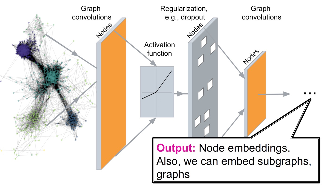
Deep encoder는 그래프의 구조에 기반한 non-linear transformation인 layer 여러 층 쌓아 node를 인코딩하는 방법으로, graph neural network를 기반으로 한다.
이를 사용하여 다음과 같은 task에 적용할 수 있다.
- Node classification
- 주어진 노드의 category(class)를 예측한다.
- Link prediction
- 두 노드가 연결되었는지 예측한다.
- Community detection
- dense하게 연결된 노드들의 cluster를 알아낸다.
- Network similarity
- 두 (sub)graph가 얼마나 비슷한지 알아낸다.
위 그림과 같이 graph network를 Deep neural network 구조에 통과시켜서 node embedding(prediction)을 만들고 싶지만, 어려운 부분이 많다.
Image는 grid 형태(=fixed size graph), Text/speech는 sequence 형태(=line graph)로 정형화되어 있으나, graph는 사이즈가 제각각이고, topological structure가 복잡하다.

Node에는 정해진 순서나 기준점(0,0)이 없으며, dynamic하거나 multimodal feature를 담는 경우도 있다.
Deep Learning for Graphs
먼저, 용어를 정리해보자.
Graph \(G\)에 대해,
- \(V\) : vertex(node) set을 나타낸다.
- \(\mathbf{A}\) : adjacency matrix (binary라 가정, 즉 연결된 노드는 1, 연결 안됐으면 0)
- \(v \in V\) : node \(v\)
- \(N(v)\) : node \(v\)의 neighbor nodes set
- \(\mathbf{X} \in \mathbb{R}^{m \times \vert V \vert}\) : node feature matrix
- Node feature examples
- Social network : user profile, user image
- Biological network : gene expression profiles, gene functional information
- Graph dataset에 node feature가 없을 때에는 node의 one-hot encoding vector(indicator vector)로 node feature를 나타낸다.
- Node feature examples
Naive Approach
Deep learning을 graph에 적용하는 가장 간단한 방법은 adjacency matrix와 feature를 결합하여 neural network에 입력해주는 것으로, 이를 naive approach라 한다.

하지만, 다음과 같은 문제가 존재한다.
- \(O(\vert V \vert)\)개의 parameter 수
- 서로 다른 size의 graph에 적용할 수 없음
- Sensitive to node ordering : 입력 행렬의 row가 node 순서에 따라 바뀐다.
Idea - Convolutional Networks
CNN에서는 grid 형태의 이미지에 대해 convolution 연산을 적용한다.
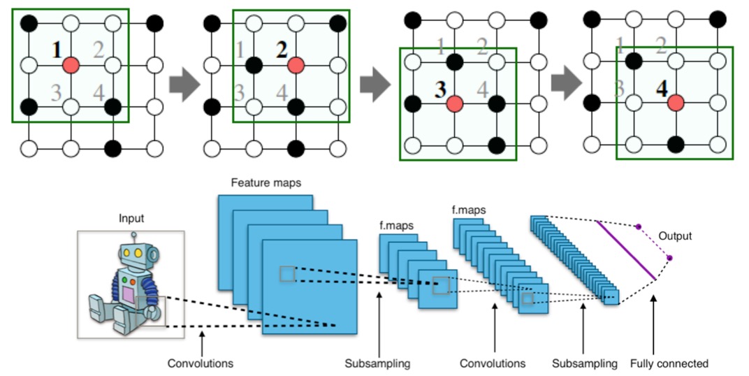
이를 graph에 적용해보면, image pixel 하나를 node로 생각해본다면 node feature/attribute에 convolution 연산을 적용해볼 수 있을 것이다.
하지만 graph는 아래와 같이 정해진 locality 개념이 없어서, sliding window를 지정할 수가 없다. (Graph는 permutation invariant이다.)

따라서, graph에서 convolutional neural network를 사용하기 위해서는 다음과 같은 아이디어를 사용한다.

Image에서의 CNN 동작은 각각 다음과 같이 graph에 적용된다.
- Filter(kernel) → target node의 이웃 노드까지를 범위로 하여 연산을 수행한다.
- Convolution operation → target node의 neighbors 및 target node 스스로의 정보를 종합한다.
- Sliding → target node를 옮겨가며 연산을 수행한다.
즉, 이웃 노드들로부터의 message \(h_i\)를 \(W_i h_i\) 형태로 transform하여 더한다. (\(\sum\limits_{i} \mathbf{W}_i h_i \))
Graph Convolutional Networks (GCN)
위 idea에 따라 target node의 이웃 노드들은 다음과 같이 computation graph를 결정한다. (\(k\)는 hop을 나타낸다.)
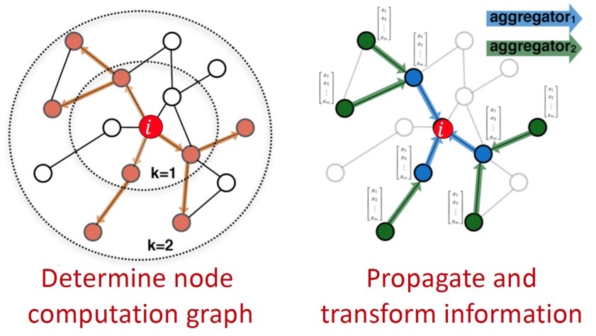
node \(i\)의 category를 예측한다고 했을 때,
- Node computation graph를 결정한다.
- Neighborhood information을 propagate 및 transform하여 aggregate한다.
이제 node feature를 계산하기 위해 정보를 전달하는 방법을 알아보자.
Aggregate Neighbors
핵심은 부분 network의 neighborhood 정보에 따라 node embedding을 생성하는 것이다.

위 예시에서 node A는 B, C, D로부터 정보를 얻는다(k=1). 그리고 각 neighbor B, C, D 또한 같은 방법으로 이웃 노드로부터 정보를 얻는다(k=2). k는 GCN에서 layer의 개념이며, computation graph에서는 hop의 개념이다.
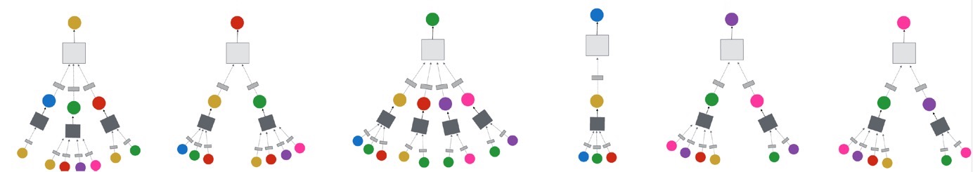
한 가지 주목할 점은, 같은 노드가 여러 번 등장할 수 있다는 것이다. 그림에서는 같은 노드처럼 보이지만, 각각 다른 feature를 갖고 있다. (위 예시에서 처음 입력된 A 노드들은 같은 feature \(\mathbf{x}_A\)를 갖고 있을 것이고, NN을 지나면서 최종 target node의 feature는 완전히 다른 상태가 될 것이다.)
이웃 노드로부터 정보를 얻을 때에는 neural network를 사용하여 aggregation을 진행한다.
Model의 depth(layer 개수)는 자유롭게 정할 수 있다.
이때, target node 각각에 대해 computation graph는 달라진다. (어떤 경우는 narrow(D)하고, 어떤 경우는 wide(C)하다.)
가장 기본적인 aggregation 방법은 negihbor들의 message를 평균낸 후에 NN을 적용하는 것이다.

수식으로 나타내면 다음과 같다.
\(\mathbf{h}_v^0 = \mathbf{x}_v\)
\( \mathbf{h}_v^{l + 1} = \sigma \left( \mathbf{W}_l \left( \sum\limits_{u \in N(v)} \cfrac{\mathbf{h}_u^{(l)} }{\lvert N(v) \rvert} \right) + \mathbf{B}_l \mathbf{h}_v^{(l)} \right), \quad \forall l \in \left\{ 0, \dots, L - 1 \right\} \)
\(\mathbf{z}_v = \mathbf{h}_v^{(L)} \)
각 term의 의미는 다음과 같다.
- \(\mathbf{h}_v^{(l)} \) : \(l\)번째 layer에서 node \(v\)의 embedding
- \(\mathbf{h}_v^0 = \mathbf{x}_v\), 즉 최초 layer embedding은 node feature로 초기화한다.
- \(\mathbf{z}_v = \mathbf{h}_v^{(L)}\) : 마지막 layer \(L\) 을 거친 후의 embedding을 나타낸다.
- \(\sigma\) : Non-linear activation function (ReLU 등 사용 가능)
- \(\sum\limits_{u \in N(v)} \cfrac{\mathbf{h}_u^{(l)}}{\lvert N(v) \rvert}\) : Aggregation 과정, 즉 이웃 노드들의 이전 layer에서의 embedding 평균
- \(\mathbf{W}_l\) : Neighborhood aggregation에 대한 weight matrix
- \(\mathbf{B}_l\) : target node 자신의 embedding vector를 transform한 것에 대한 weight matrix
다음으로, 학습을 하기 위해서는 생성된 embedding에 대한 loss function을 정의해야 한다.
위 식에서, trainable weight matrices(parameters)는 \(\mathbf{W}_l\), \(\mathbf{B}_l\)이고, node에 관계 없이 동일하다는 것을 알 수 있다. 즉, CNN의 filter처럼 노드들이 파라미터를 공유하는 것을 알 수 있다.
여느 Deep Neural Network 학습 과정과 같이, 최종 layer를 거친 결과인 final node embedding \(\mathbf{z}_v\)로 loss를 계산한 후, SGD 등의 optimizer로 위 weight parameter들을 학습한다.
Matrix Formulation of GCN
Aggregation 과정(특히, GCN에서는 average 연산)을 효율적으로 학습하기 위해서는 수식을 Matrix 연산으로 나타내는 것이 좋다.
Layer \(l\)에서의 모든 node에 대한 hidden embedding set을 \(\mathbf{H}^{(l)} = \left[ \mathbf{h}_1^{(l)}, \dots, \mathbf{h}_{\lvert V \rvert}^{(l)} \right]^\top \)와 같이 matrix로 나타내자.
이 행렬에서 \(i\)번째 행은 \(i\)번째 node의 embedding을 나타내게 된다.
따라서 embedding의 합은 adjacency matrix \(\mathbf{A}\)를 사용하여 아래와 같이 행렬의 곱으로 표현할 수 있다.
\( \sum\limits_{u \in N(v)} \mathbf{h}_u^{(l)} = \mathbf{A}_{(v,:)}\mathbf{H}^{(l)} \)
- \(\mathbf{A}_{(v,:)}\) : adjacency matrix에서 \(v\)의 이웃 노드만 1의 값을 갖는 벡터 \((1 \times \lvert V \rvert)\)
- \(\mathbf{H}^{(l)}\) : 모든 node의 embedding 행렬 \(( \lvert V \rvert \times m)\), 단 \(m\)은 embedding dimension
위 둘을 곱하면 \(v\)와 이웃한 노드의 embedding 합이 되는 것이다. 이를 \(\mathbf{A}\) 전체로 확장하면 모든 node에 대해 이웃 노드의 embedding 합을 구할 수 있다.
그리고, \(\mathbf{D}_{(v,v)} = \text{Deg}(v) = \lvert N(v) \rvert\)를 만족하는 diagonal degree matrix \(\mathbf{D}\)에 대해 inverse를 취하면 \(\mathbf{D}^{-1}_{(v,v)} = 1 / \lvert N(v) \rvert\)를 만족하게 된다.
따라서, embedding의 평균을 구하는 식은 다음과 같이 matrix로 표현할 수 있다.
\( \sum\limits_{u \in N(v)} \cfrac{\mathbf{h}_u^{(l-1)}}{\lvert N(v) \rvert} = \mathbf{D}^{-1} \mathbf{A} \mathbf{H}^{(l)} \)
간단한 예시를 통해 이해해보자.
다음과 같은 그래프가 있다.
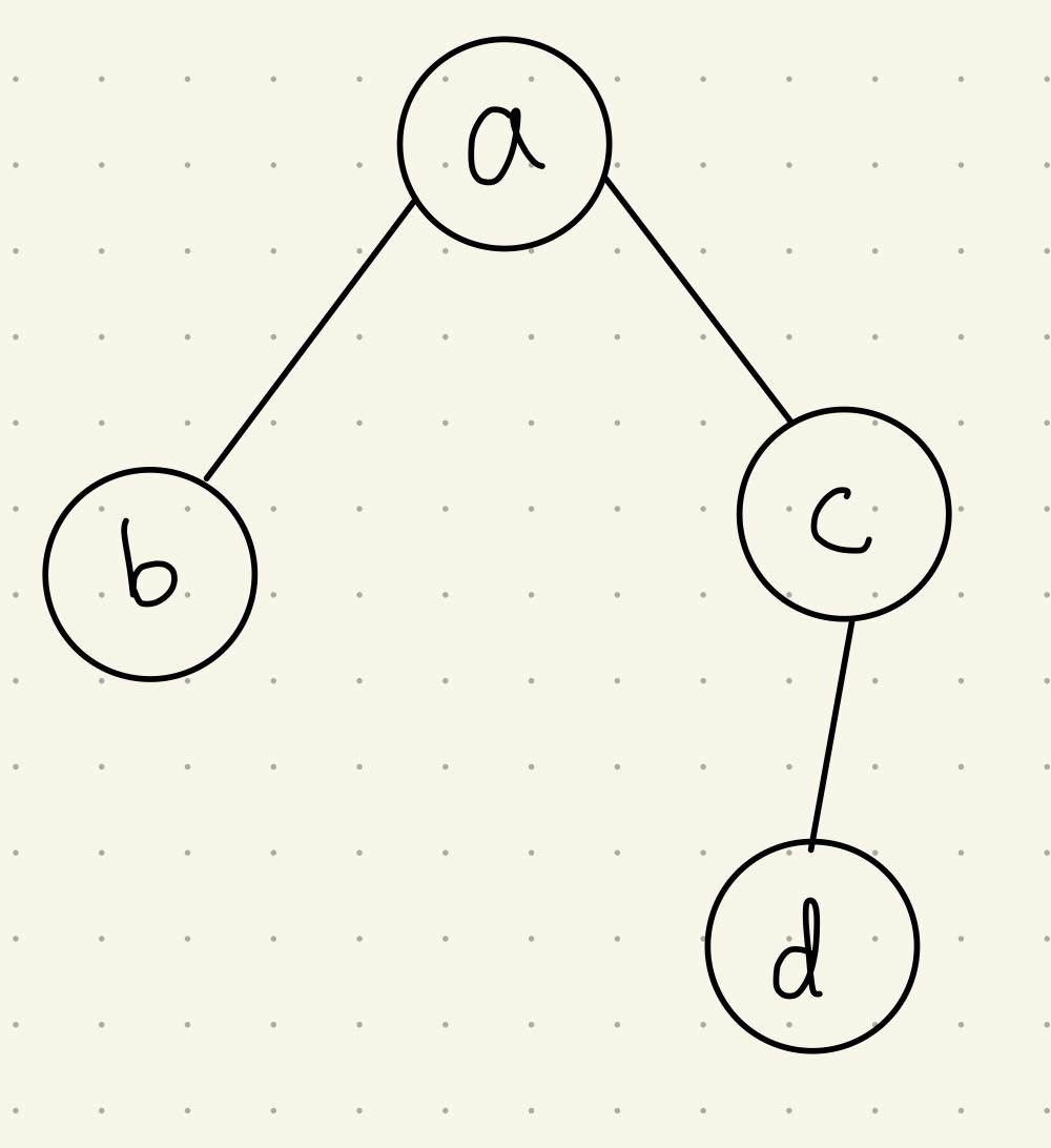
여기서 adjacency matrix는 \(\mathbf{A} = \begin{bmatrix} 0 & 1 & 1 & 0 \\ 1 & 0 & 0 & 0 \\ 1 & 0 & 0 & 1 \\ 0 & 0 & 1 & 0 \end{bmatrix}\)일 것이고, embedding matrix는 \(\mathbf{H} = \begin{bmatrix} \mathbf{x}_a \\ \mathbf{x}_b \\ \mathbf{x}_c \\ \mathbf{x}_d \end{bmatrix}\)라 가정한다.
node \(a\)에 대해 해보면, \(\mathbf{A}_{(a, :)} = \begin{bmatrix} 0 & 1 & 1 & 0 \end{bmatrix}\)에 대해 다음을 만족한다.
\( \mathbf{A}_{(a, :)} \mathbf{H} = \mathbf{x}_b + \mathbf{x}_c \)
모든 노드에 대해 확장하면, 다음 식을 얻는다.
\( \mathbf{AH} = \begin{bmatrix} \mathbf{x}_b + \mathbf{x}_c \\ \mathbf{x}_a \\ \mathbf{x}_a + \mathbf{x}_d \\ \mathbf{x}_c \end{bmatrix} \)
그리고 \(\mathbf{D}^{-1} = \begin{bmatrix} \cfrac{1}{\lvert N(a) \rvert} & 0 & 0 & 0 \\ 0 & \cfrac{1}{\lvert N(b) \rvert} & 0 & 0 \\ 0 & 0 & \cfrac{1}{\lvert N(c) \rvert} & 0 \\ 0 & 0 & 0 & \cfrac{1}{\lvert N(d) \rvert} \end{bmatrix} \)에 대해, 최종적으로 다음을 만족한다.
\( \mathbf{D}^{-1} \mathbf{AH} = \begin{bmatrix} \cfrac{\mathbf{x}_b + \mathbf{x}_c}{\lvert N(a) \rvert} \\ \cfrac{\mathbf{x}_a}{\lvert N(b) \rvert} \\ \cfrac{\mathbf{x}_a + \mathbf{x}_d}{\lvert N(c) \rvert} \\ \cfrac{\mathbf{x}_c}{\lvert N(d) \rvert} \end{bmatrix} \)
이를 통해 최종 update function은 행렬로 다음과 같이 나타낸다.
\( \mathbf{H}^{(l + 1)} = \sigma \left( \tilde{\mathbf{A}} \mathbf{H}^{(l)} \mathbf{W}_l^\top + \mathbf{H}^{(l)} \mathbf{B}_l^\top \right) \)
여기서 \(\tilde{\mathbf{A}} = \mathbf{D}^{-1} \mathbf{A}\)이며, \(\tilde{\mathbf{A}} \mathbf{H}^{(l)} \mathbf{W}_l^\top\) 부분은 neighborhood aggregation, \(\mathbf{H}^{(l)} \mathbf{B}_l^\top\) 부분은 self transformation이다.
\(\tilde{\mathbf{A}}\) matrix가 sparse하기 때문에, 계산 과정이 효율적이다. 이를 efficient sparse matrix multiplication이라 한다.
주의할 점은, aggregation function이 복잡할 경우 GNN을 matrix form으로 나타낼 수 없다는 것이다.
How to Train a GNN
학습 과정을 계속해서 살펴보자.
앞서 언급했듯이, training 대상은 learnable parameter인 matrix \(\mathbf{W}\)와 \(\mathbf{B}\)이다. 이에 대한 loss function은 task에 따라 달라진다.
1. Supervised Learning
Supervised learning에서는 다음 loss를 minimize한다.
\( \underset{\boldsymbol{\Theta}}{\min} \mathcal{L} \left(\mathbf{y}, f(\mathbf{z}_v) \right) \)
- \(\mathbf{y}\) : node의 label
- \(\mathbf{y}\)가 real number(regression task)일 경우 \(\mathcal{L}\)은 L2 norm, \(\mathbf{y}\)가 categorical value(classification task)일 경우 \(\mathcal{L}\)은 cross entropy 등이 될 수 있다.
주요 task 중 하나인 node classification task를 예로 들면, Cross entropy loss를 적용하여 다음과 같은 loss function을 얻는다.
\( \mathcal{L} = \sum\limits_{v \in V} y_v \log{\left( \sigma(\mathbf{z}_v^\top \boldsymbol{\theta} ) \right)} + (1 - y_v) \log{\left( 1 - \sigma(\mathbf{z}_v^\top \boldsymbol{\theta}) \right)} \)
- \(y_v\) : node의 class label이다.
- \(\mathbf{z}_v^\top\) : Encoder의 output인 node embedding을 나타낸다.
- \(\boldsymbol{\theta}\) : Classification weight를 나타낸다.
2. Unsupervised Learning
Unsupervised learning에서는 node label이 없으므로, graph structure를 supervision으로 사용한다.
주요 task는 node embedding이다. 비슷한 노드는 비슷한 embedding을 가지도록 학습하므로, 다음과 같은 loss를 설정한다.
\( \mathcal{L} = \sum\limits_{\mathbf{z}_u, \mathbf{z}_v} \text{CE}\left(y_{u,v}, \text{DEC}(\mathbf{z}_u, \mathbf{z}_v) \right) \)
- \(y_{u,v}\) : node \(u\)와 \(v\)가 비슷하면 1, 아니면 0의 값을 갖는다.
- \(\text{CE}\) : cross entropy
- \(\text{DEC}\) : inner product 등의 decoder (embedding 사이의 similarity)
Node similarity로는 이전 포스팅에서 살펴봤던 Random walks(node2vec, DeepWalk, struc2vec), Matrix factorization, Node proximity in the graph 등을 사용할 수 있다.
Model Design: Overview
Model을 설계하는 과정을 요약하면 다음과 같다.

1. Negihborhood aggregation function을 정의한다.
2. Embedding에 대한 loss function을 정의한다.
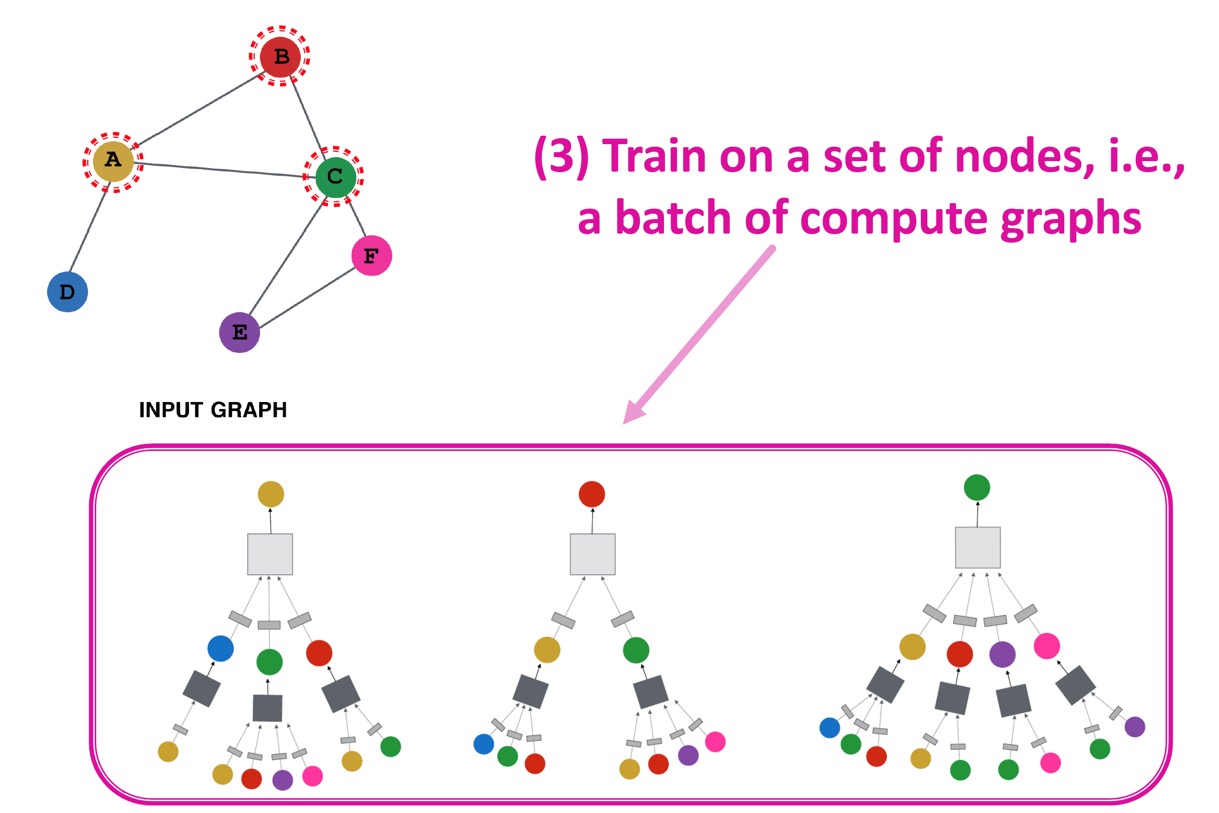
3. Node set(즉, computation graph batch 하나)에 대해 학습을 진행한다. 위 예시에서는 A, B, C node에 대한 computation graph에 대해 학습을 진행했다.
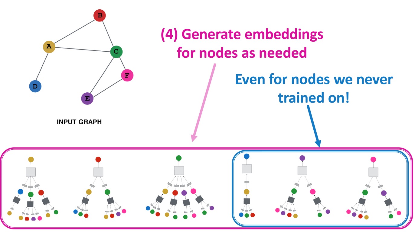
4. 필요한 node에 대한 embedding 뿐만 아니라, training하지 않은 node에 대한 embedding도 생성할 수 있다.
Inductive Capability (Parameter Sharing)
위에서 4번과 같이 training하지 않은(본 적 없는) node의 embedding도 생성할 수 있는 이유는 어떤 노드에 대한 computation graph건 상관 없이 같은 parameter \(\mathbf{W}_l, \mathbf{B}_l\)을 공유(parameter sharing)하기 때문이다. 이러한 특성을 inductive capability라 한다.
이는 본 적 없는 graph에 대해서도 똑같이 적용될 수 있다. 예를 들어, organism A를 나타내는 protein interaction graph로 학습한 모델을 사용하여 organism B의 embedding을 생성할 수 있다.
Summary
요약하자면, GNN Layer 하나에서는 이전 노드로부터의 message를 얻어와서, 이를 aggregation하는 과정을 거치고, 이러한 layer를 여러 번 쌓아 최종적으로 node embedding을 얻는다.
이를 실체화(instantiation)하기 위한 방법에 따라 GCN, GraphSAGE, GAT 등의 세부 모델이 정해진다.
그 중에서도 Graph convolutional network는 aggregation 과정에 average 연산을 사용한다.
GraphSAGE
이제까지는 message를 aggregate할 때 average 연산을 사용했다. Average 연산 대신, 더 좋은 방법을 고안하여 사용한 모델이 GraphSAGE이다.
GraphSAGE에서는 좀 더 일반적인(target node의 이웃 노드들의 vector set을 특정 vector로 맵핑하는 미분 가능한 함수) aggregation을 적용하여 다음과 같은 message passing formulation을 사용했다.
\( \mathbf{h}_v^{(l+1)} = \sigma \left( \left[ \mathbf{W}_l \cdot \text{AGG}\left( \left\{ \mathbf{h}_u^{(l)}, \forall u \in N(v) \right\} \right), \mathbf{B}_l \mathbf{h}_v^{(l)} \right] \right) \)
우선, 모든 layer의 결과 embedding인 \(\mathbf{h}_v^{(l+1)}\)에 L2 normalization을 적용하여 embedding vector의 scale을 맞춰준다.
\(\mathbf{h}_v^k \leftarrow \cfrac{\mathbf{h}_v^k}{\lVert \mathbf{h}_v^k \rVert_2}, \quad \forall v \in V \)
여기서 L2 norm은 \(\lVert \mathbf{u} \rVert_2 = \sqrt{\sum_i \mathbf{u}_i^2 }\)을 말한다.
Normalization 결과 모든 embedding의 L2 norm이 같아질 것이다.
Neighborhood Aggregation
기존(GCN)의 간단한 neighborhood aggregation과 GraphSAGE의 aggregation을 비교해보자.
먼저 기존에는 이웃 노드의 embedding 평균을 사용했다.
\( \mathbf{h}_v^{(l+1)} = \sigma \left( \mathbf{W}_l \sum\limits_{u \in N(v)} \cfrac{\mathbf{h}_u^{(l)}}{\lvert N(v) \rvert} + \mathbf{B}_l \mathbf{h}_v^{(l)} \right) \)
이에 반해 GraphSAGE는 일반화된 aggregation function을 사용한다.
\( \mathbf{h}_v^{(l+1)} = \sigma \left( \left[ \mathbf{W}_l \cdot \text{AGG}\left( \left\{ \mathbf{h}_u^{(l)}, \forall u \in N(v) \right\} \right), \mathbf{B}_l \mathbf{h}_v^{(l)} \right] \right) \)
여기서 \(\text{AGG}\)는 다음과 같은 함수를 적용할 수 있다.
Mean (Weighted average of neighbors)
Mean을 사용할 경우 기존과 같은 식을 갖게 된다.
Pool
Neighbor vector들을 MLP로 transform하여 symmetric vector function(element-wise mean/max pooling)을 적용한다.
\( \text{AGG} = \gamma \left( \left\{ \text{MLP}(\mathbf{h}_u^{(l)}), \forall u \in N(v) \right\} \right) \)
LSTM
LSTM을 적용하면 이웃 노드들을 reshuffle하는 효과를 얻는다.
\( \text{AGG} = \text{LSTM} \left( \left[ \mathbf{h}_u^{(l)}, \forall u \in \pi \left( N(v) \right) \right] \right) \)
여기서 \(\pi\)는 permutation(순열)을 의미한다.
Reshuffling을 통해 노드에 random 순서를 부여한다.


최근댓글