Autoregressive (Generative) Models (1)

이번 포스팅에서는 생성 모델 중 하나인 autoregressive model에 대해 알아보자.

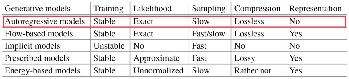
다음은 다양한 deep generative model 의 비교 표이다.

Fig 1. Comparison of deep generative models

Autoregressive Models

Autoregressive model(ARM)은 말그대로 autoregressive, 즉 이전 input data를 활용하여 현재 input과 관련된 연산(modeling probability distribution)을 하는 방법으로 \(p(\mathbf{x})\)를 모델링한다.

\( p(\mathbf{x}) = p(x_0) \prod\limits_{i=1}^D p(x_i | \mathbf{x}_{<i} ) \)

\(\mathbf{x}_{<i}\) : \(i\)번째 인덱스 이전의 \(x\)들을 말한다.

이는 이미지로 따지자면 이전 픽셀 정보를 통해 주어진 픽셀을 예측하는 개념으로 볼 수 있다. 그런데 모든 \(i\)에 대해 \(p(x_i |\mathbf{x}_{<i})\)를 모델링하는 건 사실상 불가능하다. 그래서 이를 모델링하기 위해 아래와 같은 여러 neural network를 활용한다.

Modeling with MLP

예를 들어 conditional model의 메모리가 한정되어있어 각 variable이 이전의 두 개 variable까지만 dependent하다고 가정하자(finite memory).

\(p(\mathbf{x}) = p(x_1) p(x_2 | x_1) \prod\limits_{i=3}^D p(x_i | x_{i-1}, x_{i-2}) \)

가장 간단히 MLP로 \(p(x_i)\)를 예측해볼 수 있다. \(\mathcal{X} = \{0, 1, \dots, 255\}\)라 하면, MLP는 아래와 같이 \(x_{i-1}, x_{i-2}\)를 input으로 받고, \(x_i\)의 categorical probability distribution \(\theta_i\)를 출력할 것이다.

\( [x_{i-1}, x_{i-2}] \rightarrow \operatorname{Linear}(2, M) \rightarrow \operatorname{ReLU} \rightarrow \operatorname{Linear}(M, 256) \rightarrow \operatorname{softmax} \rightarrow \theta_i \)

\(M\) : hidden unit 개수

이러한 방법으로 non-linear하면서도 parameterization이 쉬운(학습할 weight이 적은) 모델을 고안해볼 수 있다. 하지만, memory가 한정적이라는 단점이 있다. 실제로는 long-range memory가 필요한 경우가 매우 많다. (예를 들어, 이미지에서의 픽셀 수만 따져봐도 이전 두 개 정보로는 성능이 매우 떨어질 것이다.)

Modeling with RNN

따라서 MLP 대신 RNN을 활용해볼 수 있다. 그러면 conditional distribution은 다음과 같이 모델링할 수 있다.

\( p(x_i | \mathbf{x}_{<i}) = p(x_i | \operatorname{RNN}(x_{i-1}, h_{i-1})) \)

\(h_i = \operatorname{RNN}(x_{i-1}, h_{i-1})\) : hidden state

즉, history \(\mathbf{x}_{<i}\)가 계속해서 길어지므로 이에 대한 summary 개념인 hidden state \(h_i\)를 두어 이를 recursive하게 update하는 개념이다.

RNN

RNN을 간단히 복습해보자.

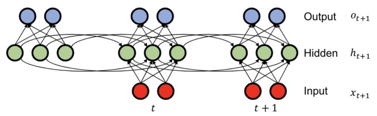
Summary update : \(h_{t+1} = \operatorname{tanh}(W_{hh} h_t + W_{xh} x_{t+1} ) \) → (time step \(t\)까지의 'summary' 개념)
Prediction : \(O_{t+1} = W_{hh} h_{t+1}\) → \(o_{t-1}\)으로 conditional \(p(x_t | x_{<i})\)의 parameter 결정
Summary initialization : \(h_0 = \mathbf{b}_0\)

이를 통해 long-range memory에 대해 간단하게 parameterize할 수 있으나, 다음과 같은 문제점을 갖는다.

Sequential : 학습이 매우 느리다.
Gradient vanishing or exploding : Weight matrix의 eigenvalue가 1보다 크거나 작은 경우 RNN이 갖는 단점으로, 결국 long-range dependency를 놓치기 쉽다.

Modeling with CNN

이러한 단점을 해결하기 위해 CNN을 활용해볼 수 있다. 특히 sequential data를 다루기 위해서는 1차원 convolutional layer, 즉 Conv1D를 활용한다.

CNN을 활용하면 다음과 같은 장점이 있다.

Parameter sharing : Kernel을 공유하므로 parameterization에 효율적이다.
Parallel computation : 연산을 parallel하게 할 수 있어 효율적인 계산이 가능하다.
Layer를 많이 쌓아 network를 깊게 구성할 수 있다.

하지만, 일반적인 Conv1D를 autoregressive model에 사용할 수는 없고, causal convolution을 사용해야 한다. Causal이란 단어는 Conv1D layer가 이전 \(k\)개 input에 dependent하다는 의미이다.

위 사진에서 첫 번째 CausalConv1D layer의 kernel size는 2이고, 두 번째와 세 번째는 각각 dilation(연산을 진행하는 간격의 개념)을 2, 3으로 적용하였다.

CausalConv1D (A)와 (B)의 차이는 각각 \(d\)번째 variable을 포함하는지 (이전 \(k\)개에 현재 input까지 dependent한지) 아닌지이다. 당연히 위에서 주어진 conditional distribution \(d\)번째(위 식에서는 \(i\)) probability를 예측하는 데 \(x_d\)는 포함되면 안될 것이다.

이러한 원리를 WaveNet, PixelCNN 등에서 활용한다.

Examples of Autoregressive Models

Autoregressive model의 예시를 좀 더 자세히 알아보자.

Fully Visible Sigmoid Belief Network (FVSBN)

Bernoulli 분포를 따르는 conditional variables \(X_i | X_1, \cdots, X_{i-1}\)가 있다고 하자. 그러면 \(x\)는 다음과 같이 예측해볼 수 있다.

\(\hat{x} = p(X_i = 1 | x_{<i} ; \boldsymbol{\alpha}^i) = \sigma \left( \alpha_0^i + \sum\limits_{j=1}^{i-1} \alpha_j^i x_j \right) \)

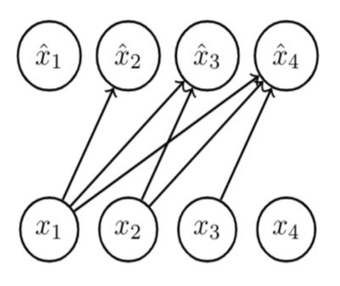
Joint distribution \(p(x_1, \cdots, x_4)\)를 구하려면, 단순히 모든 conditional(factor)을 곱해서 구한다.

\(p(X_1=0, X_2=1, X_3=1, X_4=0) = (1 - \hat{x}_1) \cdot \hat{x}_2 \cdot \hat{x}_3 \cdot (1 - \hat{x}_4)\)

\( = (1 - \hat{x}_1) \cdot \hat{x}_2 (X_1 = 0) \cdot \hat{x}_3 (X_1 = 0, X_2 = 1) \cdot (1 - \hat{x}_4(X_1 = 0, X_2 = 1, X_3 = 1)) \)

위에서 MLP를 활용한 Autoregressive model보다 더 간단하게 logistic regression을 통해 memory limit 없이 모든 이전 condition을 활용하는 모델이다.

Neural Autoregressive Density Estimation (NADE)

NADE 모델은 FVSBN의 logistic regression을 neural network(1 layer)로 바꾼 모델이다.

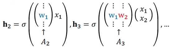
\( \hat{x}_i = p(x_i | x_{<i}; A_i, \mathbf{c}_i, \boldsymbol{\alpha}_i, b_i) = \sigma(\boldsymbol{\alpha}_i \mathbf{h}_i + b_i ) \)

\(\mathbf{h}_i = \sigma(W_{\cdot , <i} \mathbf{x}_{<i} + \mathbf{c})\) : Neural network (1 layer)

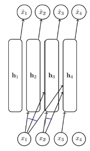
\(W_{\cdot , <i}\)는 \(A_i\)에 해당하는 weight vector를 쌓은 matrix로, \(i-1\)개의 열을 갖는 matrix가 될 것이다. (반대로 \(\mathbf{x}\)는 \(i-1\)개의 행을 가질 것이다.)

\(A\)만 고려하면 \(\mathbf{h}_i\)는 각각 parameter를 \(i\)개씩 가질 것이므로, 총 복잡도는 \(1 + 2 + \cdots + n \), 즉 \(O(n^2)\)이다. 하지만 \(W\)를 통해 이전 weight vector를 공유하여 사용함으로써 n에 대해 선형 복잡도(\(O(n)\))를 갖는다.

General discrete distributions

만약 random variable \(X_i\)가 binary distribution이 아니라 pixel intensity(0~255까지의 정수값)처럼 discrete random variable이라면, \(\hat{\mathbf{x}}_i\)를 아래와 같이 categorical distribution으로 parameterize한다. 예를 들어, random variable을 \(X_i \in \{1, \cdots, K\}\)라 가정하자.

\( \hat{\mathbf{x}}_i = (p_i^1, \cdots, p_i^K) = \operatorname{softmax}(W_i \mathbf{h}_i + \mathbf{b}_i) \)

\(p(x_i | x_{<i}) = \operatorname{Cat}(p_i^1, \cdots , p_i^K)\) : Categorical distribution
\(\mathbf{h}_i = \sigma \left( W_{\cdot, <i} \mathbf{x}_{<i} + \mathbf{c} \right)\)

위(binary distribution)에서보다 일반적인 distribution을 모델링하는 것이다.

Real-valued Neural Autoregressive Density Estimation (RNADE)

RNADE는 NADE의 variants 중 하나로, Gaussian distribution(즉 \(X_i\)가 continuous random variable, 예를 들면 음성 신호 등)을 활용한다.

\(\hat{x}_i\)가 다음과 같이 continuous distribution을 parameterize한다고 해보자. (여러 개(\(K\))의 Gaussian을 더한 형태)

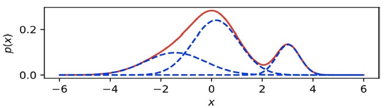
이때 \(p(x_i | \mathbf{x}_{<i})\)는 다음과 같이 모델링할 수 있다.

\( p(x_i | x_1, \cdots, x_{i-1}) = \sum\limits_{j=1}^K \cfrac{1}{K} N(x_i ; \mu_i^j, \sigma_i^j) \)

또한 앞에서와 마찬가지로 neural network로 \(\hat{x}_i\)를 나타낼 수 있다.

\( \mathbf{h} = \sigma(W_{\cdot, <i} \mathbf{x}_{<i} + \mathbf{c}) \)

\( \hat{x}_i = (\mu_i^1, \cdots , \mu_i^K, \sigma_i^1, \cdots, \sigma_i^K) = f(\mathbf{h}_i) \)

여기서 \(\hat{x}_i\)는 K개 Gaussian 각각의 평균, 표준편차 \((\mu^j, \sigma^j)\)를 정의한다. (표준편차 값을 확실히 양수로 만들기 위해 \(\operatorname{exp}\)를 취하기도 한다.)

저작자표시 비영리 변경금지

Autoregressive (Generative) Models (1)